Linear Regression Explained, Step by Step
Linear regression is one of the most famous algorithms in statistics and machine learning. In this post you will learn how linear regression works on a fundamental level. You will also implement linear regression both from scratch as well as with the popular library scikit-learn in Python. You will learn when and how to best use linear regression in your machine learning projects. You do not need any knowledge prior to reading this article.
Share on:

Background image by Christina Spiliotopoulou (link)
Outline
You’ve probably heard about linear regression before. Maybe you have even used it in a project before. And maybe, like I when I first learned about it, you had some open questions in mind as to how linear regression works in detail and why exactly we use this or that. If this is you, then you have found the right post. In this article, we’ll walk through linear regression step by step and take a look at everything you need to know in order to utilize this technique to its full potential. You’ll also understand what exactly we are doing when we perform a linear regression. We’ll go through the intuition, the math, and the code. Let’s begin!
The Main Idea
Imagine we have a dataset of houses for a specific city, where we are given the number of bedrooms for each house as well as the price of each house. The dataset might look like this:
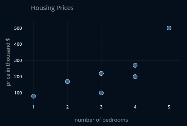
Now let’s say there is a new house for sale in the city. Wouldn’t it be cool if we could use this existing dataset to somehow predict how much the new house will cost? We can do so by trying to create a straight line
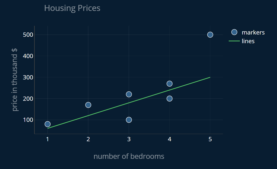
Now, if a new house enters the dataset, all we need to do is take the number of bedrooms in that house and read off the price that our line marks at that specific number of bedrooms. In other terms, we plug the number of bedrooms into our linear function and what we receive is the estimated price:
Let’s say our function looks like this
where x is the number of bedrooms in the house. Our function estimates that a house with one bedroom will cost 60.000$, a house with two bedrooms will cost 120.000$, and so on. If we plot our function alongside our data points, we get the graph above.
Looks good! But we could have also chosen this function:
or this one:
In general, we could take any function that has this form:
where determines how steep our function is and determines the value of our function at x=0. is also called the slope of our function and is called the intercept-term (because it determines the value at the point where our function intercepts with the y-axis).
We can create three plots and display them side by side:
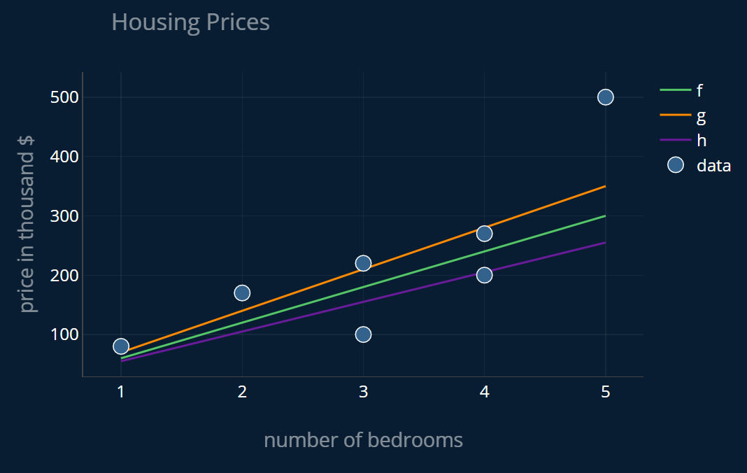
But how can we tell which of these three functions best represents the trend of our data? I mean sure, if we have a function like , we can tell that it is off, but can we somehow quantify how good or bad a specific function is? Yes, we can!
Finding the Least Squares
Ok, so we want to find out how well our line matches our data points. In other terms, we want to know how similar, or how close our line is to our points. So let’s just calculate the difference between every data point and the value of our function at that point and sum those differences together. So if we have a data point that tells us there was a house on sale with 3 bedrooms for a price of 200.000$, but our function suggests a price of 180.000$, the difference is 20.000$. And now we do this for every point.
Mathematically, we can write this sum down as:
where is the actual price of the house in thousand dollars, is the number of bedrooms in a house, and is the price our function predicts for that number of bedrooms. So if we plug in the values from our dataset, we get:
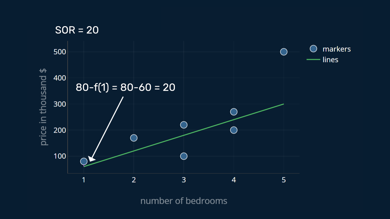
These individual differences are also called residuals. Let’s call the resulting sum the sum of residuals (or SOR for short).
At this point it might be helpful to visualize this process, so let’s take a look at it in action. At the top of the animation, we will keep track of the total SOR while we add each residual one by one.
The problem with the SOR
Now there is one problem with this. You might have noticed that when we calculate the difference of a data point and our prediction, we get a negative value if our prediction is higher than the data point. This happens when the blue data points lie below our green line.
In this case, our SOR gets reduced instead of increased. Not good! This way, individual terms might cancel each other out and our result is distorted. We want to track overestimates as well as underestimates, but right now this is not working as intended. So how can we fix this?
The first workaround that comes to mind would be to just take the absolute value, like this: . Let’s call this the sum of absolute residuals (SOAR). An alternative would be to square each term instead, like this: . Let’s call this the sum of squared residuals (SOSR).
SOAR vs SOSR
In practice, the SOAR is used a lot more rarely than the SOSR. There are a few reasons for this. The reason that is most commonly mentioned is that we avoid using the SOAR because taking absolute values makes the derivative of a function more complicated
We need to take the derivative of our metric if we want to find it’s minimum, i.e. the value with the lowest SOAR. Since the SOAR tells us how bad a function performs, we are interested in finding the lowest possible value of it, and therefor we need the derivative of it. We won’t look at derivatives in this post, but they are needed for finding the normal equation or performing gradient descent. We will take a look at these two techniques later on in the post.
Now we could try and correct our SOSR by taking the square root of every residual. But the thing is, not “correcting” our SOSR might actually be beneficial. Why is that?
If we compare the SOSR with the SOR, you might say: squaring the residuals yields a different result than the one we actually wanted, doesn’t it? We wanted to calculate the sum of residuals, but if we square each term, then large residuals increase in size a lot more than small residuals! If we have three residuals , and and we square these terms, we get , and . decreased, while increased 10-fold and increased 40-fold! This can’t be a good thing, can it? Well, in our case it actually is!
We use the SOSR to measure how well (or rather how poorly) a line fits our data. By squaring the residuals we magnify the effect large residuals have on our SOSR. This just means that we care more about large residuals than we do about small residuals. Let’s say we have two scenarios.
- In the first scenario, we have three residuals, . If we square them we get .
- In the second scenario we only have one residual, .
is exactly , so the total error of the first three residuals is exactly the same as the error of the fourth residual. The SOSR in scenario 1 would be . However, the SOSR in the second case would be . The large residual has a weight three times larger than the three smaller residuals, even though their total error is exactly the same! If we were to take the SOAR instead, we would get: .
As we see, squaring the residuals puts more weight onto large errors and less weight on smaller errors.
So when minimizing the SOSR, we always take care of the largest residual first. In contrast, when minimizing the SOAR, we treat each residual equally.
And most of the time, this property of the SOSR is a good thing. Making lots and lots of small errors is usually better than making one huge error. There is a lot more depth to this, and the topic of squares vs. absolutes appears again in another context, namely ridge and lasso regression. If you are interested in reading more about this specific topic, I recommend you take a look at the article Ridge and Lasso Regression Explained, Step by Step, where I explain this topic in its full depth. But now back to our linear regression.
Since the SOSR is the default metric, linear regression is often also called least squares regression, since our goal is to find the function that minimizes the squares in our SOSR.
Let’s evaluate our functions
Ok, great, so now we have a procedure that gives us a concrete number (or error) for every function, telling us how bad it is at predicting house prices in our dataset. Now let’s calculate these values for our three functions , and . For this let’s quickly implement our three functions as well as our SOSR in Python, so we don’t have to do the math by hand:
def f(x):return 60*xdef g(x):return 70*xdef h(x):return 45*x + 5def sosr(data,function):sosr = 0for (x,y) in data:residual = y - function(x)sosr += residual**2return sosr
We can model our dataset as a simple list of tuples (number of bedrooms, price) in Python, like this:
data = [(1, 80), (2, 170), (3, 100), (3, 220), (4, 200), (4, 270), (5, 500)]
If we now call sosr on our dataset and each of our functions , and we get:
>>> sosr(data,f)53400>>> sosr(data,g)42200>>> sosr(data,h)94875
Adjusting the SOSR
So it looks like the function best fits our data! Now I don’t know about you, but I’m a bit unhappy with our metric, the SOSR. I mean, it’s a good metric, but we can’t really interpret a SOSR of 42200. If we did not have the SOSR-values for and , how could we tell if a SOSR of 42200 is very good, decent, bad, or terrible? If we take the square root of 42200, we get ~205. This means that our function made a total error of roughly 205.000$. Now that’s pretty bad! But this number is a bit tricky to interpret. An error of 205.000$ is really bad if we only predicted the price of 7 houses, but what if we predicted 70.000 houses instead? Then this error suddenly doesn’t look that bad anymore.
Let’s therefor slightly modify our metric. After we sum the squares of every residual, let’s also divide the final result by the number of data points in our dataset. In other words, let’s take the mean (or the average) of the SOSR instead of the SOSR. This way, we don’t get the combined squared error, but instead we get the average squared error per point. And that is a lot easier to interpret. Lets take a look:
def mean_sosr(data,function):sosr = 0for (x,y) in data:residual = y - function(x)sosr += residual**2mean_sosr = sosr / len(data)return mean_sosr
Now if we use the mean_sosr to evaluate our functions we get:
>>> mean_sosr(data,f)7628.571428571428>>> mean_sosr(data,g)6028.571428571428>>> mean_sosr(data,h)13553.57142857143
and if we take the square root of each value, we get:
>>> sqrt(mean_sosr(data,f))87.34169352933013>>> sqrt(mean_sosr(data,g))77.64387566686395>>> sqrt(mean_sosr(data,h))116.41980685678631>>>
This means that on average, made an error of ~87.000$, an error of ~77.000$ and an error of ~116.000$ for each prediction. Now that’s a lot more intuitive if you ask me! We get a very intuitive feel for the size of the error our functions make. If our function predicts some price we know that, on average, that price can be off by up to 77.000$. Of course, this is just a rough estimate, but it still helps to get a more direct feel for how good our bad our functions are. And most importantly, we know that an average error of 77.000$ is pretty bad! And we can see this without having to compare multiple functions to each other.
Clearing Things Up
Ok, so there are a few things that I want to address at this point to make everything as clear as possible. First and foremost, let’s fix our naming conventions.
Fixing the Names
SOAR, SOSR, and mean SOAR might be very descriptive names, but they are not used in practice. Usually, we use more general terms. In practice, the mean SOSR (mean sum of squared residuals) is just called the MSE (mean squared error)
Why not just take the Square Root?
Ok, we do take the square root to interpret our MSE, so why don’t we include the square root into our metric directly? We could, and it can be helpful at times. The resulting metric would be called the root mean squared error or RMSE and it is sometimes used in practice. But using the RMSE instead of the MSE would not really help us out a lot. But why?
First of all, this would again just make our math more complicated. And if we can keep our metric simple, that’s usually a good idea, because a simpler function means a simpler derivative, which means we can compute it faster. Also, we would mostly undo the effect which weighs large values more heavily than small ones, which we mentioned earlier. In this case we actually want to weigh large errors more heavily, which is another reason to just stick with the MSE. Would the RMSE still work though? Yes, it would. But why make things more complicated when the simpler option already does everything we want?
Apart from that, it is also nice to know that a value which minimizes a certain function also minimizes the square root of the function .
This is why taking the RMSE instead of the MSE would also work to solve our linear regression problem.
Ok, now that we have these things cleared up, let’s continue with finding the best possible line for our data!
Finding the Best Function: Visualize
Before we think about how to find the best possible function, let’s first think about how this function would behave or in other terms, which properties it should have.
We have said that we can use any function that has the following form:
for some and some . We then defined our evaluation metric to be the MSE. The MSE for our specific case is defined like this:
where our data contains tuples of the shape . We can assume that our data is constant since we are only looking at our particular dataset. This means that our MSE only depends on the function . And our function only depends on and , since ist just our input data. With those aspects in mind, we can rewrite our MSE as such:
The part in blue is equal to . Because our s and our s are constant, our MSE now only depends on the two variables (or model parameters) and .
What we can do now is we can visualize this definition of our MSE for every value of and . This results in a three-dimensional plot, where we have on the x-axis, on the y-axis, and our MSE on the z-axis.
The resulting plot looks like this:
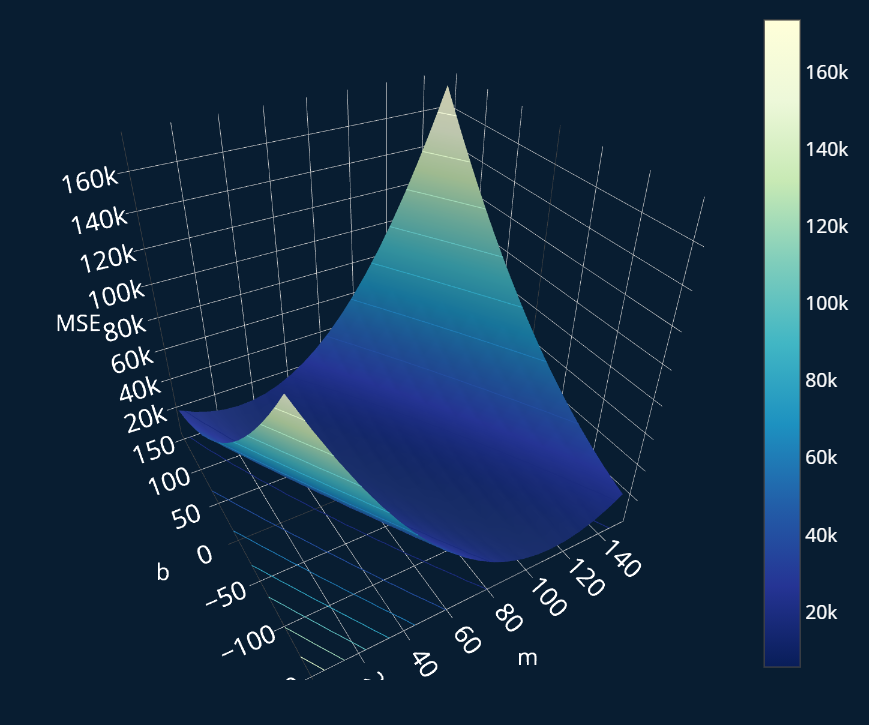
Ok, that looks neat! Our final goal is to find the function, that for some and some has the lowest MSE. In this plot, we can see the MSE for every and every . Thus, if we can find the lowest point on this surface (i.e. the minimum), we get the lowest possible MSE! And then all we have to do is take the values of and for that minimum, plug them into our function, and we’ve solved our linear regression! Ok, that’s the plan. But how do we find this minimum, without having to go through every possible value for and ?
I want to present you with two different ways for how we can compute our ideal function.
Finding the Minimum: Normal Equation
Linear regression as a problem is simple enough (mathematically speaking), that we can compute a function that gives us the ideal values for our and our directly. This means that we only have to solve one single equation, and we’re done. When something like this exists, we say that there is a closed-form solution for our problem. The corresponding function is then called a normal equation. Before we take a look at the normal equation though, let us first vectorize our MSE. We don’t have to do this, but doing this not only makes the normal equation look much neater, but it also makes this procedure easier and more efficient to implement.
Adjustment: Vectorization
We defined our MSE like this:
There is nothing wrong with that definition, but if we wanted to translate our definition into code,
what we would probably do is create a loop that sums up each of the individual residuals.
This is exactly how we’ve implemented our mean_sosr-function.
For our small dataset of 7 points that is no big deal, but imagine we had 100.000 data points (which is not uncommon today).
Every time we wanted to compute our MSE, we would have to perform 100.000 operations through our loop. We can do better than this!
For this, we will vectorize our equation. This has the benefit that we can use NumPy to perform our calculations, and NumPy is a lot faster than just a regular Python loop!
Vectorization is worthy of its own post, which is why I have created a separate article
where I explain in detail what vectorization and its benefits are and how we can vectorize
our linear function as well as the MSE. I would highly recommend you give it a read, but if you want to keep things short, here’s what we do in a nutshell.
We will rewrite our definition of the MSE
to this:
where is equal to:
where and are defined as:
In code, our new implementation will look like this:
def mse_vectorized(y, y_predicted):error = y-y_predicted # save y-y_pred in a variable so that we only have to compute it onceloss = 1/(y.size) * np.dot(error.T, error)return loss
If you are interested in how we arrive at this new definition, I encourage you to read the corresponding article, where we go through this particular example step by step. It should only take about 7 minutes to read, so if you are interested, take a look and then return to this post afterward.
With the vectorization now cleared up, let’s finally take a look at the normal equation.
The Normal Equation
The equation looks like this:
where is the optimal parameter vector , meaning it contains the parameter values that minimize our MSE. The in means we are transposing . Loosely speaking this just means that we swap the rows and columns with each other in our . The after the brackets on the left means we take the inverse of the matrix that is calculated inside of the brackets.
Getting to this normal equation requires a bit more math
Implementing the Normal Equation
With that being said, we can simply implement this equation in Python like this:
def normal_equation_linear_regression(x,y):intercept_ones = np.ones((len(x),1)) # results in array( [ [1],..,[1] ] )x_b = np.c_[intercept_ones,x] # we now add the additional ones as a new column to our Xtheta_optimal = np.linalg.inv(x_b.T.dot(x_b)).dot(x_b.T).dot(y) # the normal equationreturn theta_optimal
In the first line of our function, we create this array:
array([[1.],[1.],[1.],[1.],[1.],[1.],[1.]])
In the second line, we combine this newly created array with our x.
We do this by using numpy’s c_-operator. This will take our X_b and our intercept_ones
and concatenate them along the second dimension. What this means is that it will add our ones as a new column.
The resulting array will look like this:
array([[1., 1.],[1., 2.],[1., 3.],[1., 3.],[1., 4.],[1., 4.],[1., 5.]])
Lastly, we compute our normal equation. np.linalg.inv computes the inverse of our matrix,
whereas .T transposes the matrix it is being called on. The .dot-operator is just a multiplication, meaning X_b.T.dot(X_b)
is equal to .
Ok, now let’s plug these values into our function and see what values we get, shall we?
dataset = np.array([(1,80),(2,170),(3,100),(3,220),(4,200),(4,270),(5,500)])x = dataset[:,0]y = dataset[:,1]
>>>normal_equation_linear_regression(x,y)array([-46.31578947, 84.73684211])
Ok, that looks like something. Let’s also calculate the MSE for those values:
def f_ideal(x_b):return np.dot(x_b,[-46.31578947, 84.73684211]) # -46.31578947 + x * 84.73684211>>>mse(x,f_ideal(x))5691.72932330827
That looks pretty good! The square root of 5691 is ~75, which means that our ideal function is off by “only” about 75k$ per estimate. Now that still does not sound that great, but it is a lot better than any of our initial functions , and, . If we display this point (-46.32, 84.74) on our three-dimensional plot, we get this:
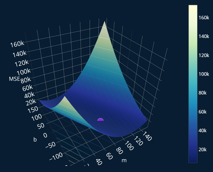
Indeed, it really is the minimum!
Now we have learned how we can solve any linear regression problem in just a few lines of raw Python code and we also took a look at the math behind it.
Using Scikit-Learn
We can achieve the same result by using the popular library scikit-learn.
Scikit-learn provides a LinearRegression-class we can use for this.
But before we can do that, we have to make a small adjustment to our data.
Scikit-learn expects our x to be two-dimensional (since, in most cases, we will have more than one feature),
but right now our x is only one-dimensional. So we redefine our x like this:
x = np.array([[1], [2], [3], [3], [4], [4], [5]])y = np.array([ 80, 170, 100, 220, 200, 270, 500])
and now we can solve our linear regression problem like this:
from sklearn.linear_model import LinearRegressionlinreg = LinearRegression()linreg.fit(x,y)
To inspect our variables, we can simply run:
>>>print(linreg.coef_,linreg.intercept_)[84.73684211] -46.31578947368433
As we see, scikit-learn got exactly the same result as our own code. Nice!
Our Final Line
Let’s now finally take a look at our optimal line:
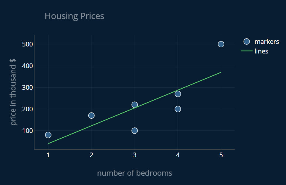
We can also plot our line directly in Python with the following matplotlib-code:
import matplotlib.pyplot as plty_predict = [f_ideal(i) for i in x]plt.plot(x, y_predict, "g-") #g- means: use green as the color ("g"), and draw a line ("-")plt.plot(x, y, "b.") #b. means: use blue as the color ("b"), and draw individual points (".")plt.show()
Cool! As you see, the points lie pretty close to our line, except for the last point. Our mathematical formula gave us the optimal solution, but maybe we can still ask ourselves if we can somehow do better? The answer is maybe. You may have noticed that our last data point seems a bit off. I added this point on purpose. This last point is a so-called outlier, a value that significantly distances itself from the average value at that point. There are a number of different ways we can handle outliers and if you want to learn more about them, I recommend you read my article Outliers in Data and What You Can Do To Fix Them, where I explain in detail how you can find outliers and what you can do to stop them ruining your machine learning model. For now though, we can be happy that we found our ideal function!
Finding the Minimum: Gradient Descent
Another way to find our ideal function takes a completely different approach. Instead of directly computing the ideal values for our variables, we instead approach them step by step. In a nutshell, gradient descent starts with a random function and continuously improves it until it can no longer be improved.
I think Aurélien Géron described the idea behind the algorithm with a great analogy in his book “Hands-On Machine Learning with Scikit-Learn, Keras & TensorFlow”, so I will share it with you here.
Imagine you are on the side of a hill and you want to get to the valley. But the air is very foggy. So foggy, that you can only see the ground you are standing on and nothing else. But you can still feel the slope of the hill, right? So by taking very small and cautious steps in the downward direction, you will eventually reach the valley. This is in essence how gradient descent works.
Gradient descent is worthy of its own post, so I will not go into further detail here. If you are interested in reading more about how we can use gradient descent to solve our linear regression, I recommend you read Gradient Descent for Linear Regression Explained, Step by Step, where I go into much more detail and show you step by step how we can use this method to find the function that best fits our data.
Complexity
To finish off this post let’s talk a bit about complexity. If there are multiple ways to solve our linear regression problem, how can we decide on which one we should use? Let’s perform a small complexity analysis for this.
When we solve our normal equation, we have to compute . is an matrix where is the number of our features and is the number of samples in our dataset. So for our , which looks like this:
our will be 2 and our will be 7. The second dimension is instead of , because we add the 1 to every sample to account for our bias term. If we transpose an matrix, we get an matrix. Multiplying these two matrices together gives us a matrix.
Inverting this matrix has a time complexity somewhere between and because there are multiple ways to compute the inverse of our matrix. The complexity therefor depends on the specific implementation. This means that if we double the number of features (or input parameters) that we have, we multiply our computation time by a factor between and . This is very costly.
The other operations in this equation are all matrix multiplications, which have a complexity of at most . As we see, solving the normal equation has a very bad time complexity with regard to , the number of features (it’s between quadratic and cubic) and a pretty good time complexity with regard to , the number of entries in our dataset (it’s linear!).
With gradient descent, we only perform one small step at a time. This means that the complexity of the closed-form solution comes from very few large operations, whereas the complexity of gradient descent comes from very many small operations. Performing one iteration of gradient descent is therefor fairly cost-efficient. The cost of gradient descent comes from performing many of these small steps.
So how do we choose between the two?
If our dataset is very large, as long as it fits in our memory, solving the normal equation won’t be too difficult. But if we have large number of features, things will get ugly.
At some amount of features, solving the normal equation will no longer be feasible, and it becomes more efficient to use gradient descent instead and iteratively approach the ideal solution, rather than computing it directly. So if you have to choose between these two, you can decide based on the number of features in your dataset.
However, most of the time
when you want to use linear regression,
you dataset will likely not have 1000+ features. If it does,
then you are most likely trying to solve a rather complicated problem with machine learning,
in which case there might be an even better tool to use than linear regression.
This means that most of the time you
will be just fine using scikit-learn’s LinearRegression-class.
Let’s look at how Scikit-Learn handles this, shall we?
What does Scikit-Learn use?
Scikit-learn uses yet another technique for its LinearRegression-class: Singular Value Decomposition (or SVD for short).
The complexity of this approach is roughly . This means that with regard to the number
of entries in our dataset, we still have a linear time complexity. But this approach is a bit faster
with regard to the number of features in our dataset. Explaining exactly how SVD works in the
context of linear regression would make this already long post even longer. If you are interested
in reading more about this though, let me know in a comment below so that I know there is demand
for this! If you want to use gradient descent for solving a linear regression problem with
scikit-learn, you can use the SGDRegressor-class instead.
Below you can see a plot that shows how many computations we have to perform for specific amounts of input parameters.
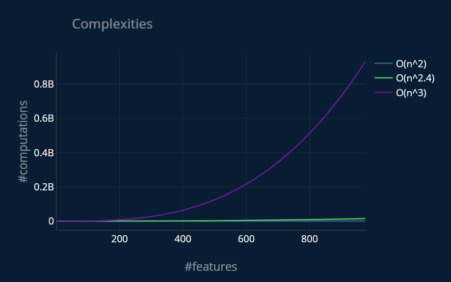
You can click on the labels in the top right to toggle the individual graphs on and off. As you see, the differences between the complexities are massive! Because of this, it is crucial that you choose the right method to solve your linear regression problem.
Further Reading
If you have made it this far, congratulations! This post was quite long and I hope you now understand linear regression intuitively, mathematically, visually and are also able to solve linear regression problems using raw Python code as well as with the help of scikit-learn.
I know this can be a lot to take in when you are just starting out, and if you feel like you need some time to go through all of this step-by-step, then that is absolutely fine.
This was also the first post where I heavily integrated these custom interactive visualizations. I would love to know what you think of them! Let me know your opinion in the comments below, I would really value it.
Continuing in the Same Direction
If you still can’t get enough of linear regression, I would highly recommend you read the post Lasso and Ridge Regression Explained, Step by Step next. Lasso and ridge are basically variations of linear regression and if you understand linear regression, lasso and ridge should not be to difficult too understand as well.
Outside the Box
In this article, we looked at an exemplary application of linear regression on a small dataset with one feature (the number of bedrooms) and one target, also called label (the price of the house). Of course, you could also use more than just one feature for linear regression! You could f.e. predict the price of a house based on the number of bedrooms, the number of restrooms, the age of the house, and so on. In this example, we also did not transform our dataset in any way and directly used it to train our model. Sometimes, you can achieve even better results by transforming the data first. You could f.e. square the number of bedrooms for each house before plugging them into your linear function. Doing something like this is called feature engineering, which is where you pick and modify the features that should be used to train your machine learning model. If this sounds interesting to you, then I recommend you take a look at the category Dataset Optimization, where you’ll find articles explaining topics such as feature engineering, outliers, and much more!
Share on:
