Lasso Regression Explained, Step by Step

You have probably heard about linear regression. Maybe you have even read an article about it. Lasso and ridge regression are two of the most popular variations of linear regression which try to make it a bit more robust. Nowadays it is actually very uncommon to see regular linear regression out in the wild, and not one of its variations like lasso or ridge. The purpose of lasso and ridge is to stabilize the vanilla linear regression and make it more robust against outliers, overfitting, and more. Lasso and ridge are very similar, but there are also some key differences between the two that you really have to understand if you want to use them confidently in practice. This article is the second article in a series where we’ll take a deep dive into ridge and lasso regression! We will look at how we might have come up with lasso regression ourselves, distinguish it from ridge regression, and we’ll also code it up in Python. Let’s start!

This article is a direct follow up to the article Ridge Regression Explained, Step by Step, so ideally you should read the article about ridge regression before you read this article. In the linked article, we construct ridge regression from scratch and go through all of the details necessary to understand ridge. Since lasso is very similar to ridge, we’ll use a similar approach in this post. However, this article will be a lot more fast-paced since the details have already been covered in the article about ridge. So I highly recommend you read that article first, before coming back to this one. With that being said, let’s take a look at lasso regression!

So what is wrong with linear regression? Why do we need more machine learning algorithms that do the same thing? And why are there two of them? We’ve explored this question in the article about ridge regression. Here’s a quick recap:

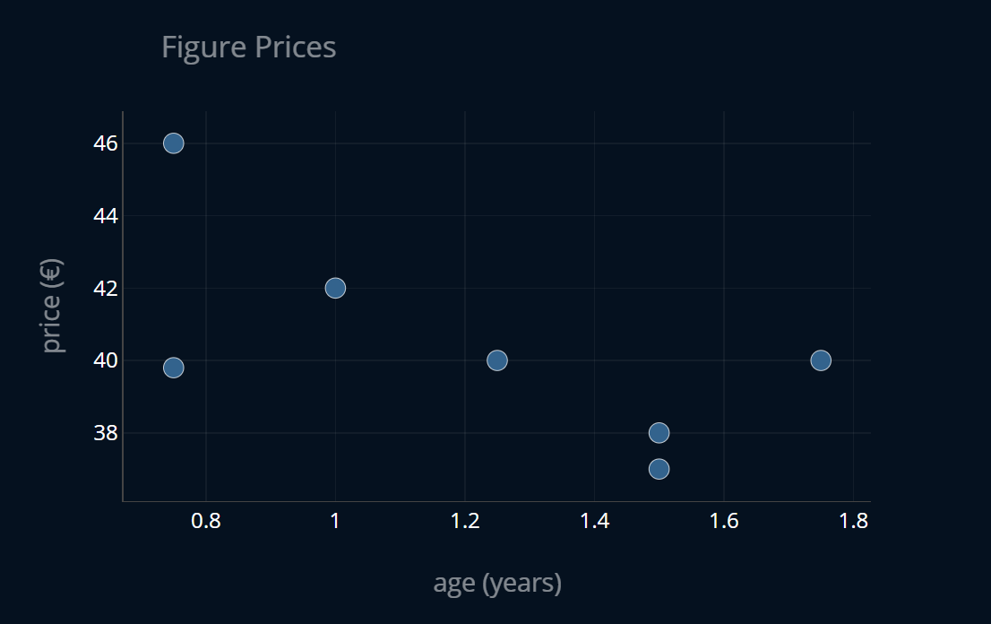
We had a dataset of figure prices, where each entry in the dataset contained the age of the figure as well as its price for that age in € (or any other currency). We then wanted to predict the price of a figure given its age using linear regression, to see how much the figures depreciate over time. The dataset looked like this:

We then split our dataset into a train set and a test set and trained a linear regression (OLS regression) model on the training data. Here’s how that looked like:

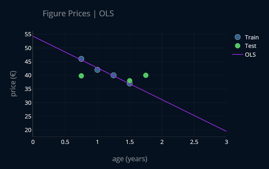
We then noticed that this model had a very low training error but a rather high testing error and thus we concluded that our linear regression model is overfit. We then tried to come up with an imaginary, better model that was less overfit and looked more like this:

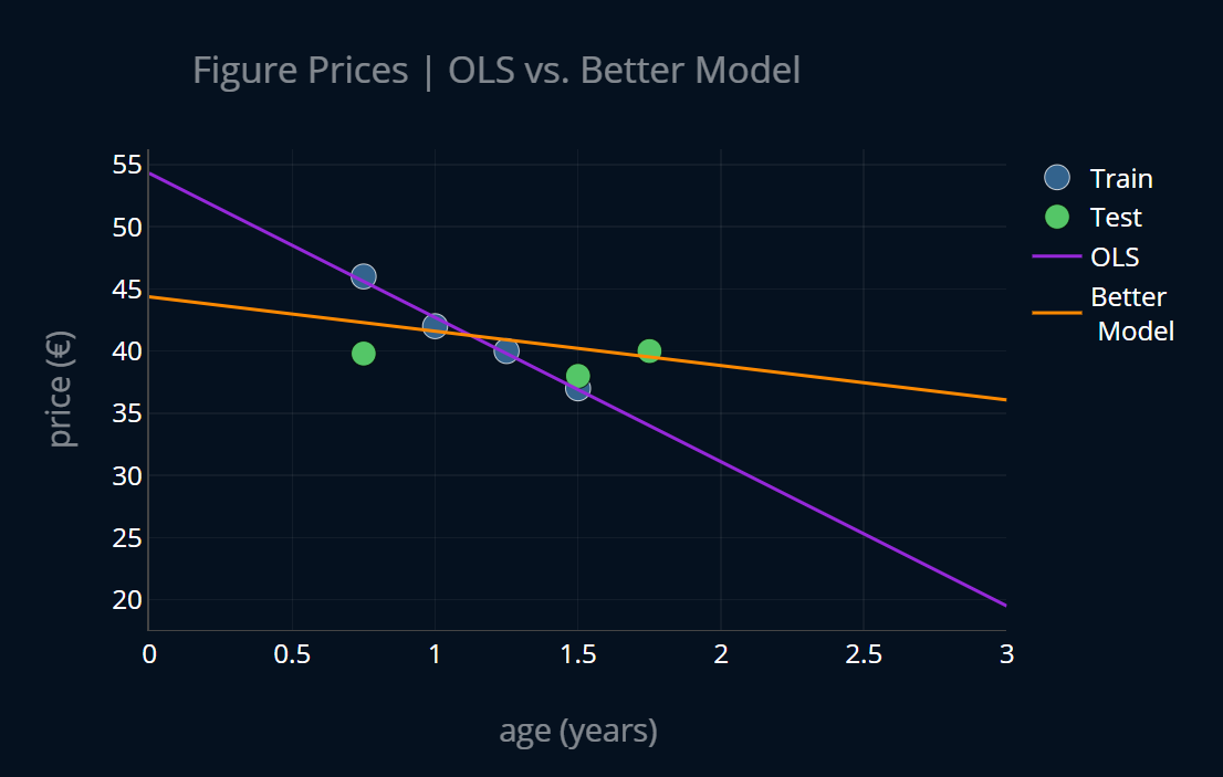
This imaginary model turned out to be ridge regression. We analyzed what exactly lead to our linear regression model overfitting and we noticed that the main cause of overfitting were (absolutely) large model parameters. After discovering this insight, we developed a new loss function that penalizes large model parameters by adding a penalty term to our mean squared error. It looked like this (where $m$ is the number of model parameters):

There’s just one problem with this loss function. Since our model parameters can be negative, adding them might decrease our loss instead of increasing it. In order to circumvent this, we can either square our model parameters or take their absolute values:

The first function is the loss function of ridge regression, while the second one is the loss function of lasso regression. In this article, we will focus our attention on the second loss function.

If you are familiar with norms in math, then you could say that the lasso penalty is the $l_1$-norm (or Manhattan norm) of our parameter vector $\boldsymbol{\theta}$. This is also the reason why this term is sometimes referred to as an L1 regularization. This means that we can rewrite our new loss like this (a norm is denoted using two vertical lines, like this: ||):

In the article about ridge regression, we also went on and visualized the difference between OLS regression and ridge regression. Since the visuals don’t change a lot for lasso, we’ll skip this part for now. We know the mathematical difference between ridge and lasso, but what does this difference mean in practice?

When should you choose lasso over ridge (and vice versa)? Are there any differences in practice? Do lasso and ridge produce identical models? Let’s try to answer these questions by looking at a concrete example. We will assume that we have some linear model with added regularization. Our linear model has the parameter vector $\boldsymbol{\theta}$ with the following values:

Now let’s say that as part of some regularization procedure, we want to reduce the size of our model parameters. For simplicity purposes, let’s assume that we’ll only change one of the parameters at a time. What happens when we use ridge and lasso regression, respectively? Let’s look at both cases.

Ridge

The ridge penalty is $||\boldsymbol{\theta}||_2^2 = \boldsymbol{\theta}^T\boldsymbol{\theta}$, so in our case this would be:

If we reduce the first parameter by 1, our penalty will now look like this:

This means that by reducing our first model parameter from 10 to 9, we reduced our ridge penalty by 19, from 125 to 106. If we instead decreased the other parameter by 1, we would get this penalty:

This means that, by reducing our second model parameter from 5 to 4, we reduced our ridge penalty by 9, from 125 to 116. This is less than the reduction we got when we reduced our first model parameter!

Since the ridge penalty squares the individual model parameters, large values are taken into account much more heavily than smaller values. This means that our ridge regression model would prioritize minimizing large model parameters over small model parameters. This is usually a good thing because if our parameters are already small, they don’t need to be reduced even further. Let’s now take a look at how this situation looks like when using the lasso penalty.

Lasso

The lasso penalty is $||\boldsymbol{\theta}||_1 = \sum_{i=1}^m{|\theta_i|}$, so in our case this would be:

If we reduce the first parameter by 1, our penalty will now look like this:

This means that by reducing our first model parameter from 10 to 9, we’ve reduced our ridge penalty by 1, from 15 to 14. If we instead decreased the other parameter, we would get this penalty:

This means that by reducing our first model parameter from 10 to 9, we reduced our ridge penalty by 1, from 15 to 14. This is equal to the first reduction!

Since the lasso penalty consists of the absolute model parameters, large values are not taken into account more strongly than smaller values. This means that our lasso penalty would not prioritize minimizing any particular model parameter, unlike the ridge penalty, which prioritizes large parameters.

One consequence of this is that with ridge regression, weights can get very very small, but they will never be zero. This is because if we square a number between 1 and 0, the square will be smaller than our original number. In other words, the ridge penalty gets smaller and smaller the closer we get to zero. And this shrinking of the ridge penalty is amplified when we get closer to zero. With lasso however, this loss shrinking is constant. This is why, when we use lasso regression, some weights (more precisely, the least useful ones, because they also contribute least to minimizing the loss) might be set all the way to zero.

Let’s look at a small example. We want to predict the price of a figure based on the age of the figure, as before. But this time, we also take into account the initial price of the figure (init price), the number of figures produced in the initial year of release (#produced), the average temperature in the country the figure was manufactured in (temp), as well as the average number of pets per household in Europe (PPH). If we write this down as a function, we would have:

The age, initial price, and the number of figures produced all seem to be quite relevant features. In contrast, the average temperature and the number of pets per household seem completely irrelevant to this regression problem. How would knowing the average amount of pets per household in Europe help us predict figure prices? These last features are pretty useless in this regard. If we use ridge regression for this problem, none of the weights $\theta_1, \theta_2, \theta_3, \theta_4,$ and $\theta_5$ would be reduced to 0. They would probably be reduced to very small values, but they would not be set to 0, even though they are completely useless. However, when we use lasso regression, the weights $\theta_4$ and $\theta_5$ that control the influence of the average temperature and the number of pets per household in Europe, would be set to exactly 0. This is nice because it allows us to completely eliminate some features from our dataset and focus only on the important ones. In most scenarios, we don’t actually know which features are useful and which are not. With lasso, when a weight is equal to exactly 0, we can remove it from our dataset and our model will still perform exactly the same as before.

From this we can conclude that lasso regression is particularly well suited when we want to minimize the number of features our model should use. If we think that a lot of features in our model might be rather unhelpful for our model, then using lasso is a great choice. Conversely, if we think that most features in our dataset could be really helpful, ridge might have a slight advantage over lasso. In most cases, however, these two algorithms will produce very similar results. So which one should you choose if you don’t know anything about the usefulness of your features? Then your best bet is to just use both lasso and ridge and determine the best value for $\alpha$ using cross-validation. There is also a model called elastic net which, in a nutshell, is just OLS regression with both a ridge penalty and a lasso penalty attached to it. If you’re interested in elastic net, the third article of this series, Elastic Net Regression Explained, Step by Step, has all of the relevant details you need to know! But back to lasso. How can we actually determine what model parameters $\boldsymbol{\theta}$ we should use?

In this section of the article about ridge regression, we’ve looked at the ways to solve ridge regression. It turned out that, to solve ridge, we can just use the same techniques that we used to solve regular OLS regression. Lasso can’t be that much different, right? Well, it is, actually. The bad news is that there is no closed-form solution for lasso, meaning there is no normal equation we can solve to immediately get all of our ideal model parameters. But why? What is it about lasso that makes things more complicated?

Recall that we can derive a normal equation by finding the minimum of our loss function, i.e. differentiating it, setting it equal to zero, and then solving for our model parameters. However, our lasso penalty makes things a little bit more difficult. To understand why, let’s look at a small example. Let’s consider the simple function $f(x) = x^2$. To find the minimum of $f$, we take the first derivative of it, we set it equal to zero, and then we solve for $x$. With this we get that our minimum is at x=0, easy. Now let’s consider the following function, which is the absolute function: $g(x) = |x|$. The function looks like this:

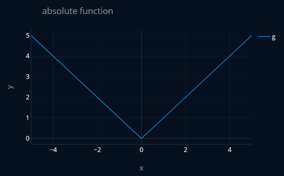
We can’t use the same approach for this function, because $g$ is not differentiable at x=0. The slope of $g$ is 1 for all values greater than 0, and -1 for all values smaller than 0. But what is the slope of $g$ at x=0? It is undefined. So we can’t actually differentiate our function $g$ at x=0.

Now back to lasso. We want to derive a closed-form solution for the lasso-MSE:

But this function also contains absolute values! Recall the sum rule for derivatives:

In the case of our lasso loss, we have a multivariate function, since our inputs $y$ and $y_{pred}$ are vectors (and because there’s two of them), but we can just use the multivariate sum rule for derivatives:

Here, $\nabla$ is the gradient-operator. The word “gradient” sounds really fancy but all that $\nabla(f)$ does is provide us with all of the partial derivatives of $x$ in a vector. Here’s a little example:

Gradients are explained in more detail in this section of the article about gradient descent for linear regresion, so if you’d like to read more about this, check out that article.

So what we’re doing here is taking the derivative of our MSE, adding that to the derivative of our lasso penalty, summing those two up, and what we get is the derivative of our lasso-MSE. The orange part in the gradient above is the derivative of our lasso penalty, which is the derivative of a sum of absolute values. As we just saw, we can’t differentiate these absolute terms for $\theta_i=0$ , so we can’t compute the gradient here!

This is the reason why there is no general closed-form solution for lasso. This is by no means a full, mathematically rigorous proof, but it should be more than enough to understand the underlying problem. So what can we do? We can’t just ignore the point at x=0, since it’s a pretty important one. We can’t compute a closed-form solution, so we’ll have to use a different method to solve lasso. In particular, we are going to use gradient descent to do so! Or rather, we are going to use some slight variations of gradient descent, because regular gradient descent also needs the gradient of our function (as the name would suggest), which, as we just saw, can’t be computed. The two most popular variations of gradient descent that are used to solve lasso are coordinate descent and subgradient descent. In a nutshell, coordinate descent updates one parameter (or coordinate) at a time, while subgradient descent uses a subgradient instead of a regular gradient, which, unlike the regular gradient, we can compute for the lasso-MSE.

When I first wrote this article, I explained both subgradient and coordinate descent, showed how to implement them from scratch and then I also visualized them. This however lead to the article taking over 40 minutes to read in it’s entirety. So instead of doing that, let’s get straight to the visuals and compare subgradient and coordinate descent on a graphical level! (Don’t worry, we’ll get back to the other parts in a moment)

Before looking at the visualizations, let’s first ask ourselves what we should be expecting. For subgradient descent, it should probably not look too different from regular gradient descent, because our subgradient will be similar to a supposed regular gradient. Below you can see a 3-dimensional plot where for every combination of input parameters $\theta_1$ and $\theta_0$ (I’ve named them m and b in the plot, to make them more easily distinguishable), the lasso-MSE is plotted. By pressing the buttons at the top, you can perform one iteration step of subgradient descent. After the first ten steps, each button press cycles through more than just one step at a time, so that you don’t have to press one button 300 times. Let’s take a look:

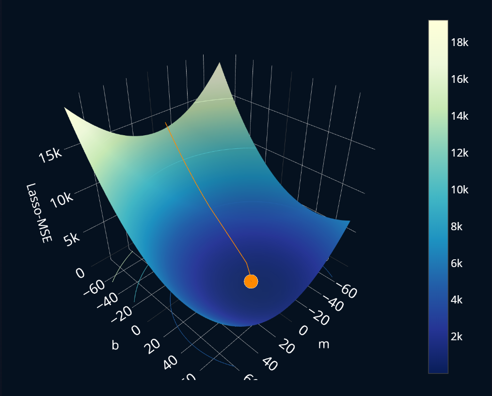
Alright, just as expected! So subgradient descent proves to be a working alternative when regular gradient descent doesn’t work. Nice! But using subgradient descent in the context of lasso regression has one fatal flaw, which is also the reason why scikit-learn only provides an implementation of coordinate descent, but not one of subgradient descent for its Lasso-class. The worst part is that in many books (even in really good ones!) this part is often overlooked when talking about subgradient descent for lasso. We’ll have to take a deeper look into subgradient descent to really understand what’s going on. So if you want to understand how subgradient descent works and why you shouldn’t use it to solve lasso regression, read the article Subgradient Descent Explained, Step by Step to find out! As far as I know, this is currently the only article on the web that covers this topic in such great detail, so it will definitely be worth your time!

Ok, but what about coordinate descent? Since we’re only looking at one coordinate at a time, the descent should look a lot more zigzaggy than regular gradient descent. Let’s again make a plot where you can click buttons to control the current iteration of gradient descent. Have a look:

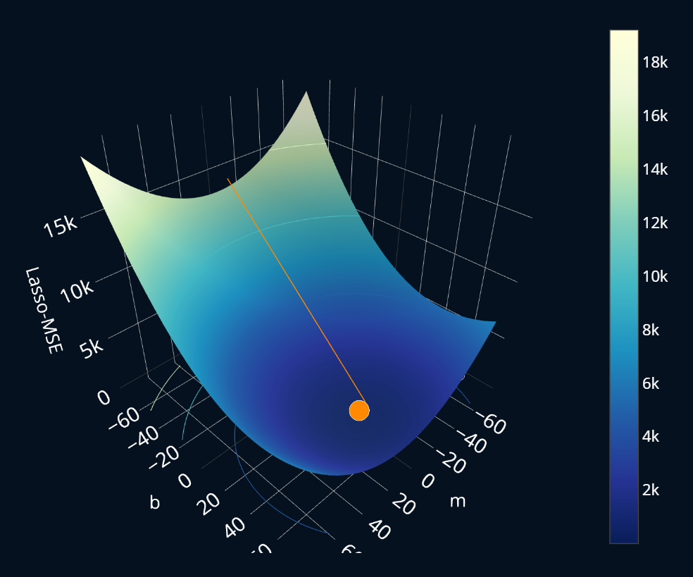
Ok, that was 1. incredibly quick and 2. somewhat zigzaggy, as expected. You can see how the first step only adjusts b and the second step only adjusts m (you might have to zoom in a bit to see it more clearly). Then there are some tiny improvements but after the first steps the minimum is already found. But why did it converge so quickly?! This makes subgradient descent look a lot worse when compared directly to coordinate descent. So what is the reason behind the speed of coordinate descent? If you want to find out how coordinate descent works, how you can implement it, and most importantly, why it is so extremely fast, you can take a deeper dive and read Coordinate Descent Explained, Step by Step. In that article, you will learn everything about how coordinate descent works, how you can implement it from scratch and why it is so incredibly fast. So Coordinate descent is basically as good as it gets.

But why did we then even look at subgradient descent if, in practice, you’ll basically always use coordinate descent? The reason is that subgradient descent is quite a bit easier to implement, and thus its implementation is a lot less prone to errors than the one of coordinate descent. This is also the reason why in almost every book and every “machine learning from scratch”-course, you will be presented with just an implementation of subgradient descent for lasso. Only sometimes is coordinate descent mentioned and even rarer is it actually implemented. This is why I have created the articles Subgradient Descent Explained, Step by Step as well as Coordinate Descent Explained, Step by Step. By reading these articles, you will understand exactly where the limits of subgradient descent are and how coordinate descent is able to perform so well. In these articles, we will also implement the mentioned algorithms from scratch, so you can truly understand how these variations of gradient descent work under the hood. I highly recommend that you give these two a read after finishing this article.

Now I don’t want to let you go without showing you some practical code, so let’s look at how we can perform lasso regression with scikit-learn (which uses coordinate descent under the hood!).

Using lasso with scikit-learn is quite simple with the Lasso-class.

But before we can perform our regression it is crucial that we standardize our data, because ridge and lasso are sensitive to the scaling of the data. If you’re interested in what can go wrong if you don’t standardize your data before using ridge and lasso, and how exactly standardization solves this problem, check out the article When You Should Standardize Your Data.

Here’s our data:

 X = np.array([1.25, 1.  , 0.75, 1.5, 1.75, 1.5 , 0.75])
 # since sklearn expects a 2d-array for our X,
 # we add an additional dimension along the first axis using the following command
 X = np.expand_dims(X,1)
 y = np.array([40. , 42. , 46. , 37., 40. , 38. , 39.8])

The first thing we do is we split our dataset into a training and testing portion:

 X_train, X_test = X_s[:4], X_s[4:]
 y_train, y_test = y[:4], y[4:]

Then we create a StandardScaler and train it using only our training dataset. All this “training” does is calculate the mean and standard deviation of our dataset and store them. Then, we standardize our X:

 from sklearn.preprocessing import StandardScaler
 
 scaler = StandardScaler()
 scaler.fit(X_train)
 X_s_train = scaler.transform(X_train)
 X_s_test = scaler.transform(X_test)

And now we can perform our regression as follows:

 from sklearn.linear_model import Lasso
 
 lasso = Lasso()
 lasso.fit(X_s_train, y_train)
 print(lasso.coef_[0], lasso.intercept_)
 # prints: -2.5269426990176953 40.63053220519125

Instead of manually standardizing our data before feeding it into our Lasso model, we can also use a so-called pipeline to dynamically standardize the data that goes into our model. This way we don’t have to duplicate our dataset in memory, which saves space. This approach would look like this in code:

 pipeline = make_pipeline(StandardScaler(), Lasso())
 pipeline.fit(X_train, y_train)
 print(pipeline[1].coef_[0], pipeline[1].intercept_)
 # prints: -2.5269426990176953 40.63053220519125

Earlier we’ve talked about how lasso regression has the ability to produce sparse model parameters. To make sure this is actually the case, we can perform a simple test. We create a completely random X, a completely random y, and then we run lasso on it. Ideally, every single parameter should be set to zero because there should be no correlation between our X and our y. Let’s try it out:

 X_rand = np.random.rand(100,50)
 y_rand = np.random.rand(100)
 
 pipeline = make_pipeline(StandardScaler(), Lasso())
 
 pipeline.fit(X_rand, y_rand)
 
 print(pipeline[1].coef_, pipeline[1].intercept_)
 # output:
 # [-0.  0. -0.  0. -0.  0. -0. -0. -0.  0. -0.  0.  0.  0. -0. -0. -0.  0.
 #   0.  0. -0. -0. -0. -0.  0.  0.  0. -0. -0.  0. -0.  0.  0.  0. -0.  0.
 #   0. -0.  0. -0.  0. -0.  0. -0.  0.  0. -0.  0. -0.  0.] 0.48078044760264155

As we can see, every weight has been zeroed out. The only exception to this is the bias (or intercept) of our lasso model. This is because scikit-learn’s lasso implementation does not regularize the bias.

Apart from Lasso, scikit-learn also provides a another class that can be used to create a lasso model, namely SGDRegressor which, as the name suggests, uses stochastic gradient Ddscent (SGD). Maybe you’re scratching your head right now. Didn’t we state that the L1 penalty is not suited for regular (stochastic) gradient descent because the absolute values are not differentiable at 0? Yes, we did. However, there are a number of methods to alter the penalty and make it suitable again. Specifically, we mentioned subgradient descent and coordinate descent. But there are even more options to choose from! Scikit-learn for example uses a truncated gradient instead of a regular gradient for its SGDRegressor-class.

This approach is similar to regular gradient descent, but the difference is that the weight updating process is divided into two steps. The first step is updating the weight without the L1 penalty. The second step is applying the L1 penalty. The trick here is that the penalty is only applied to such an extent as to not change the sign of the weight. In other words, the weight is cut off (or truncated) at zero. This happens for every weight and thus we have a truncated gradient instead of a regular one. You can read more about this particular approach in the paper by Tsuruoka et al. titled “Stochastic Gradient Descent Training for L1-regularized Log-linear Models with Cumulative Penalty”.

Let’s try it out:

 pipeline_sgd = make_pipeline(StandardScaler(), SGDRegressor(alpha=1, penalty="l1"))
 pipeline_sgd.fit(X_train, y_train)
 print(pipeline_sgd[1].coef_[0], pipeline_sgd[1].intercept_)
 # prints: -2.2233194459768386 [40.87110655]

Nice, it produces almost the same result as our Lasso model. We can also test if it produces sparse weights by fitting a SGDRegressor model on our random dataset:

 pipeline_sgd = make_pipeline(StandardScaler(), SGDRegressor(alpha=1, penalty="l1"))
 pipeline_sgd.fit(X_rand, y_rand)
 print(pipeline_sgd[1].coef_, pipeline_sgd[1].intercept_)
 # output:
 # [0. 0. 0. 0. 0. 0. 0. 0. 0. 0. 0. 0. 0. 0. 0. 0. 0. 0. 0. 0. 0. 0. 0. 0.
 #  0. 0. 0. 0. 0. 0. 0. 0. 0. 0. 0. 0. 0. 0. 0. 0. 0. 0. 0. 0. 0. 0. 0. 0.
 #  0. 0.] [0.46368558]

Nice! In general, coordinate descent will converge quite a bit faster than this truncated SGD, so in practice you should usually stick to using Lasso.

For ridge regression, scikit-learn offers RidgeCV. For lasso regression, there is LassoCV! It works in exactly the same way as RidgeCV, which we’ve explored here. Since our dataset is so small, LassoCV will throw an error if we try to fit it using our current X_train and y_train. What we can do is increase the size of our training set:

 X_train, X_test = X_s[:5], X_s[5:]
 y_train, y_test = y[:5], y[5:]

Now we can use LassoCV like that:

 lasso_cv_pipeline = make_pipeline(StandardScaler(),
                                   LassoCV(alphas=[0.1, 1.0, 10]))
 lasso_cv_pipeline.fit(X_train, y_train)
 print(lasso_cv_pipeline[1].alpha_)
 # output: 0.1

Good job on finishing this article! If you want to continue learning, here are some recommendations.

In this article, we took a look at lasso. In the previous one, we took a look at ridge. So which one should you choose? Well… I’ve never said that you have to make the choice, did I? In fact, you can use both ridge and lasso at the same time! How? We can use something that’s called elastic net. If you’re interested as to how this works, take a look at Elastic Net Explained, Step by Step. The article also has a nice summary that goes over all of the scikit-learn-classes like Ridge or SGDRegressor and explains them in an organized fashion!

In the article about ridge regression, we saw that not standardizing our data can lead to some problems. In this article, we’ve standardized our data before fitting our Lasso model. But how exactly does standardization work and why is it so important to use when dealing with regularized models? If you want to read some clear and easy-to-understand answers to those questions, head right on to the article When You Should Standardize Your Data to find out more!

In this article, we’ve looked at lasso regression, which is an adaptation of OLS regression. But like with ridge, we can also take the lasso penalty and apply it to other models, like logistic regression or polynomial regression! If you’re interested in these regularized models, I recommend you take a look at the articles Logistic Regression Explained, Step by Step and Polynomial Regression Explained, Step by Step. There you will learn everything you need about the named models as well as their regularized variants!