When, Why, And How You Should Standardize Your Data
Standardization is one of the most useful transformations you can apply to your dataset. What is even more important is that many models, especially regularized ones, require the data to be standardized in order to function properly. In this article, you will learn everything you need to know about standardization. You will learn why it works, when you should use it, and how you can do so with just a few lines of code.
Share on:
Photo by Dominik Schröder (link)
Outline
Standardization is a process from statistics where you take a dataset (or a distribution) and transform it such that it is centered around zero and has a standard deviation of one. What exactly this means, what problems standardization solves, and when you should standardize your data is exactly what you’ll learn by reading this article! A lot of models (especially ones that contain regularization) require the input data to be standardized in order to work properly. There are lots of questions on the internet about how you should correctly standardize your dataset. Should you use the entire dataset for standardization? How should you standardize new data points? What happens if I don’t standardize my data? We will answer these questions, as well as many more, in this article!
Prerequisites
You should be comfortable with at least one machine learning model, like linear regression before you read this article. Since standardization is especially important for regularized models, it also helps if you know at least one regularized model, like ridge regression. You should also be familiar with the notion of training and testing datasets. If you need a refresher on that, check out the article How to Split Your Dataset the Right Way.
Additionally, we will explore a practical example from the article Ridge Regression Explained, Step by Step to motivate the idea of standardization. So if you’d like to have a little bit more context about the setting from this article, you can consider reading or skimming the article about ridge regression. With that being said, let’s begin!
The Setting
So what’s the issue? What problem does standardization solve? What can happen if we don’t standardize our data? Let’s look at a concrete example to see where things might go wrong. If you’ve already read the article about ridge regression, then this example will feel familiar.
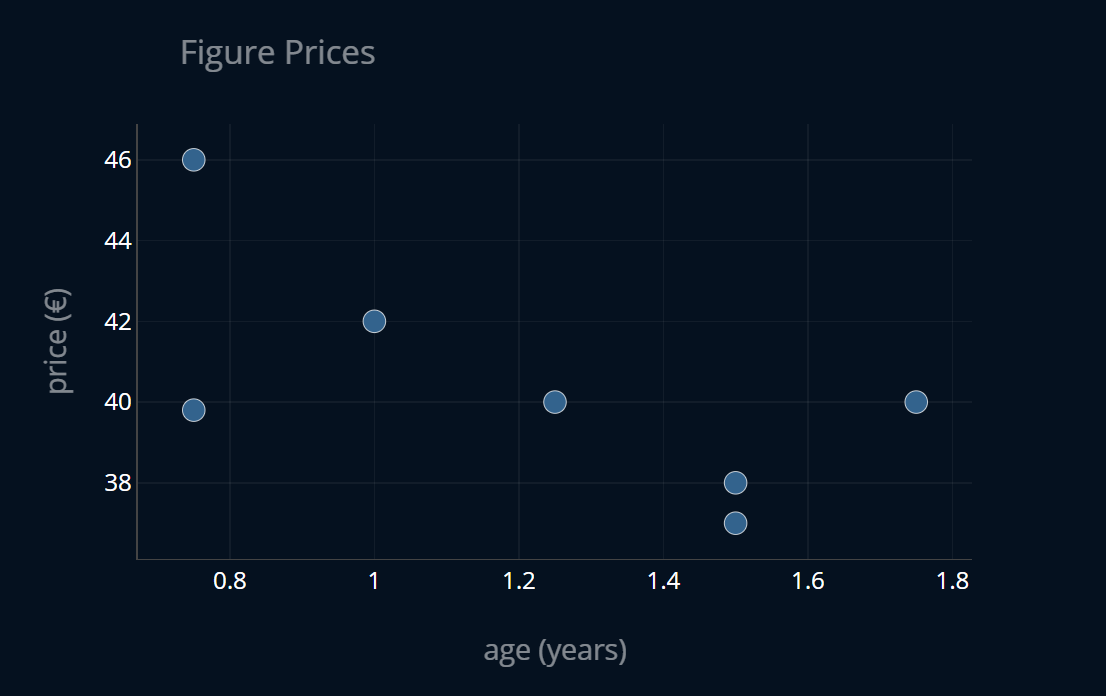
Let’s say we have a dataset of figure prices where each entry in the dataset contains the age of the figure in years as well as its price for that age in € (or any other currency). We then want to predict the price of a figure given its age using linear regression (OLS regression), to see how much the figures depreciate over time. The dataset looks like this:
We now split our dataset into a training and testing portion and create a linear regression model as well as a ridge regression model:
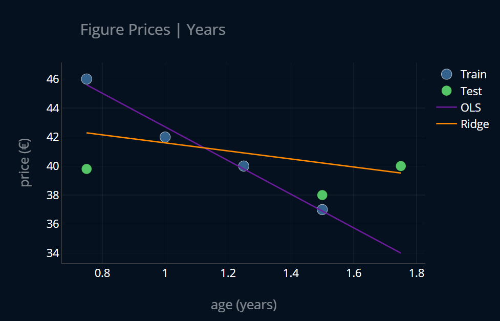
Now everything looks alright, doesn’t it? So what’s the problem?
When to Use Standardization and Why
Before we take a look at what standardization is,
let’s look at what problem it solves first.
Right now our X (our features) tells us the age of every figure in years, right?
Now what happens if we change that to
days, instead? In other words, what happens if we do this:
X_days = X * 365 # let's ignore leap years for now
and train our two models on X_days instead of X?
Our dataset will still look the same and it will still hold the same information as before,
so one would assume that our models will also look the same, right?
Before you take a look at the plot below, take a second to think about what we should expect.
Should both models remain the same? Should both change?
Let’s run our two models again and see what happens:
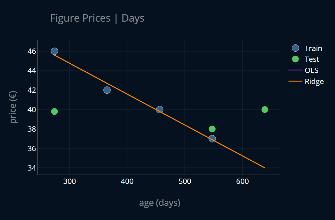
That’s interesting.. our ridge regression model now produced the same linear function as our OLS regression model!
But.. why? With X_days, we’ve put our X onto a larger scale than before. Maybe, by also putting
our X onto a lower scale and looking at the outcome, we can gain a deeper insight.
So let’s do that and create new features X_decades that describe the age of every figure not in years, but in decades.
I.e. we do this:
X_decades = X / 10
Take another second and think about how our models should look like when we train them on X_decades.
Ready? We train our models once more and we get:
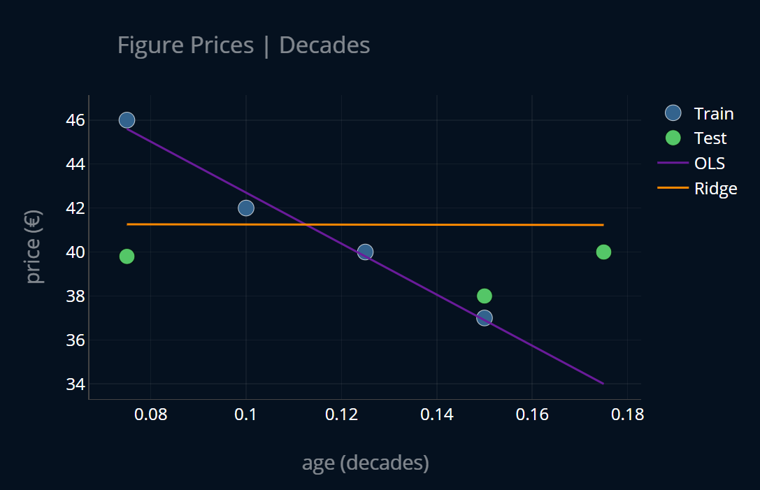
Interesting! Now our ridge regression model seems to have moved in the opposite direction, it is almost completely flat. Our OLS regression however remained unchanged. We can get some structure into these observations by plotting these three experiments side by side. Let’s also keep track of the model parameters (at the bottom of each plot). Here’s how that looks like (click on the image to zoom in!):

Ok, much better! Below every plot, you can see the model parameters in the format [intercept, slope]. There are a couple of things to note here:
- It seems that only our ridge model is sensitive to the scaling of the input data.
- The ridge penalty becomes weaker when our data points are closer
together, and stronger when they are further apart.*For example, the points in
X_daysare further apart from each other than the points inX_years. This is because two points that were apart one year are now apart 365 days. To us humans this is the same, but to the machine these are different numbers. - The slope of the OLS model increases when our points are closer together.
- The intercept term of the OLS model doesn’t change. Only the slope changes.
Let’s try to make sense of these points one by one. Point one makes sense when we recall the loss of our two models ( are our model parameters):
The loss of our OLS model is just the MSE, which does not care about the size of our model
parameters. The ridge loss, however, contains an L2-penalty, which punishes large model weights.
Now let’s take a look at the slope of our OLS regression model once more.
It is -116, which is pretty large (in the absolutes) in the plot on the right, where we use X_decades.
This makes sense because our data points are very close to each other (absolutely speaking). Each data point
is maybe 0.02 units away from the next, so our slope has to be relatively large.
But the ridge penalty discourages large model parameters! This is why our ridge model
becomes so flat in the right example.
Similarly, in the left example, where we use X_days,
the data points are pretty far apart from each other, which means that our slope
should be particularly small (in the absolutes), which is true since it is just -0.03 for OLS regression.
And the ridge penalty encourages small model parameters,
so it does not see a problem with our (now) small model parameters, so it does not regularize them further!
This issue appears very frequently in machine learning and it can be a real pain to deal with because you might not suspect that the scaling of your data is causing these issues. This issue also affects almost all regularized models, because they all share some sort of regularization term that punishes large model weights.
Here is when standardization comes into play. Standardization allows us to put all of our features on the same scale, resolving this issue. So when and why should we use standardization?
Generally speaking, standardization should be used when your model has a regularization term or is otherwise sensitive to the scaling of the input features. Standardization transforms all features onto the same scaling, thereby ensuring that regularization and other scaling-sensitive operations work properly.
Now that we know when we should use standardization and why, let’s take a look at how exactly it works.
How Standardization Works
What standardization does is it puts every feature in a dataset on the same scale. So how does it work? It involves the following two steps:
- subtract the mean (the expected value)*of the dataset from every feature pointGenerally the mean is not the same as the expected value, especially if you’re dealing with probability distributions and random variables. The expected value for a discrete random variable is the sum of every event outcome times the probability of that event occurring. In our dataset we’re not dealing with any probabilities, so we can just drop that part from our equation. The event outcome in our case is just the y-value of a data point, i.e. the price of a figure for some age. That’s why in this case the mean and the expected value are the same.
- divide every feature point by the standard deviation (std for short) of the dataset
And that’s it! In essence, you can implement standardization in just one line of code:
X_standardized = (X - np.mean(X) ) / np.std(X)
Often times you will see it being written like that:
Here, is the expected value of our dataset (which in this case is just the mean) and is the standard deviation of our dataset.
Nice!
Let’s take a look at what happens
when we standardize our X_days, our X_years, and our X_decades.
Here’s an image showing the three datasets on the left and their standardized variants on the right (For this, I visualized
the data points as bars because the plot is quite large, and bars are easier to see than points):
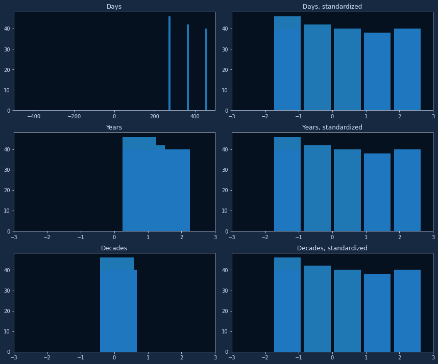
You can see how the three standardized datasets are exactly the same! We can visualize this process to better understand the two steps individually (we’ll only include the training data for now):
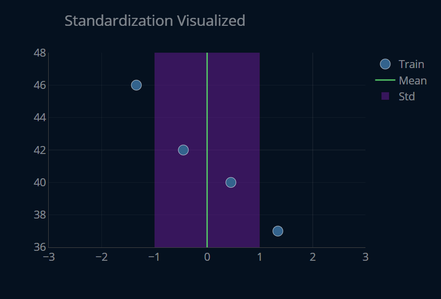
In the plot above, you can press the button at the top to perform the standardization steps.
If we now run OLS regression and ridge regression on our standardized dataset (any of the three, since they are now the same), we get:
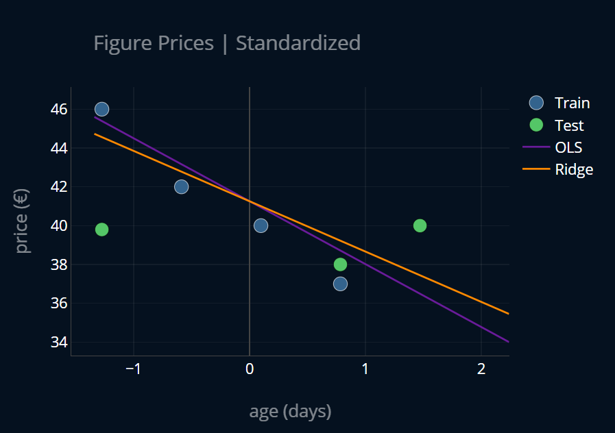
Nice! This looks quite a bit less regularized than our initial ridge model, but it just goes to show how much of a change standardization can make! Now let’s look at how we can actually implement it.
Standardizing Multiple Features
In our example, we only have one feature (the age of a figure). But standardization also works if you have multiple features! Let’s say we were given not only the age of every figure but also the number of people who have preordered that figure. Our dataset would look like this:
| Sample Index | Age (years) | #Preorders | Price (€) |
|---|---|---|---|
| 1 | 1.25 | 1000 | 40 |
| 2 | 1 | 300 | 42 |
| 3 | 0.75 | 1200 | 46 |
| 4 | 1.5 | 500 | 37 |
| 5 | 1.75 | 600 | 40 |
| 6 | 1.5 | 250 | 38 |
| 7 | 0.75 | 900 | 39.8 |
Now we want to standardize this dataset.
To do this we can just standardize every feature separately,
meaning we standardize the age-column and then we standardize
the #preorders-column. This is how we can apply standardization
when we have more than one feature. If you are using something like scikit-learn’s StandardScaler,
this will be done automatically.
How to Implement Standardization
I want to present you with three ways to implement standardization.
We can implement it 1. by hand, 2. by using scikit-learn’s StandardScaler,
and 3. by utilizing scikit-learn’s Pipeline. Let’s start with the first way.
Implementing Standardization Manually
So let’s say we have our features X. How can we standardize them?
Here’s the process:
- Split the dataset into train and test subsets (using something like scikit-learn’s
train_test_split-function) - Compute mean and std of the train set
- Standardize train and test set using the values computed in step 2
In code, it would look like this:
X_train, X_test, y_train, y_test = train_test_split(X, y, test_size=0.33, random_state=42)X_train_mean = np.mean(X_train)X_train_std = np.std(X_train)X_train_standardized = (X_train - X_train_mean) / X_train_stdX_test_standardized = (X_test - X_train_mean) / X_train_std
Then we can train and use our model as follows:
ridge = Ridge()ridge.fit(X_train_standardized, y_train)print(ridge.intercept_, ridge.coef_[0])# outputs: 40.7 -1.56ridge_predictions = ridge.predict(X_test_standardized)print(ridge_predictions)# outputs: [40.48 41.35 39.61]
Two things are important here.
- Always only use the training set to compute the mean and std, and standardize the test set using these exact values.
- Always standardize data that the model should predict using the mean and std of the training set.
Note that when we standardize our test data using the mean and standard deviation of the training data, the resulting dataset will usually not have a mean of exactly 0 and not have an std of exactly 1. That is ok. The important part is that the transformation stays consistent across training and testing sets.
Alternatively, instead of computing the mean and standard deviation ourselves,
we can use scikit-learn’s StandardScaler.
Implementing Standardization using Scikit-Learn’s StandardScaler
We can create a StandardScaler-object and train it using only our training dataset.
All this “training” does is compute the mean and std of the data we feed it and store those values
for later use.
Then we can use our scaler to standardize our testing set.
It looks like this in code:
from sklearn.preprocessing import StandardScalerscaler = StandardScaler()scaler.fit(X_train)X_train_standardized = scaler.transform(X_train)X_test_standardized = scaler.transform(X_test)
Instead of writing scaler.fit(X_train) and X_train_standardized = scaler.transform(X_train) we can also just write
X_train_standardized = scaler.fit_transform(X_train) to save us one line of code.
Now we can again train our model:
ridge = Ridge()ridge.fit(X_train_standardized, y_train)print(ridge.intercept_, ridge.coef_[0])# outputs: 40.7 -1.56ridge_predictions = ridge.predict(X_test_standardized)print(ridge_predictions)# outputs: [40.48 41.35 39.61]
The results are exactly the same.
Implementing Standardization using Scikit-Learn’s Pipeline
In the previous two examples, we had to be extra careful to always use only the training data to compute our standardization parameters (the mean and the std) and also always standardize new data that goes through our model. Because this is a bit cumbersome and very prone to errors, there is an easier solution: pipelines. Pipelines allow us to perform these computations automatically, by sequentially chaining transformations, as well as one regular machine learning model, together. They look like this:
from sklearn.pipeline import Pipelinepipeline = Pipeline([('scaler', StandardScaler()),('ridge', Ridge())])
Every item inside of a pipeline has to be a tuple containing a name as well as a transformation
(meaning it needs to implement a .transform-method), apart from the very last item, which has to be a tuple containing a name and a model.
We can then access our items like this:
pipeline["scaler"]# orpipeline[0]
When we call .fit on our pipeline, what will happen is that we will first fit our
StandardScaler and then we will transform our data using said StandardScaler.
Then we will use that transformed data to fit our ridge regression model. When we call .predict
on our pipeline, we will first transform our data using our scaler, and then use that transformed data
to make our predictions with our ridge model.
When fitting or predicting, all of the transformations are applied on the fly, saving us
the hassle of applying the transformations manually. Pipelines take care of the rules
mentioned above, saving us some lines of code and reducing the possibility of errors in our code.
There is also make_pipeline, which makes creating pipelines even easier:
from sklearn.pipeline import make_pipelinepipeline = Pipeline([StandardScaler(), Ridge()])
Here, we don’t even have to specify the names of our items, because make_pipeline will
use the lowercase types of each class as the names automatically (f.e “ridge” for Ridge).
Regardless of whether we use Pipeline or make_pipeline, the training process will be
exactly the same:
pipeline = make_pipeline(StandardScaler(), Ridge())pipeline.fit(X_train, y_train)print(pipeline[1].intercept_, pipeline[1].coef_[0])# 40.7 -1.56pipeline_predictions = ridge.predict(X_test_standardized)print(pipeline_predictions)# [40.48 41.35 39.61]
As you can see, the results of these three methods are exactly the same! make_pipeline saves us a few lines
of code and reduces the potential for errors, because it it always uses the same StandardScaler-object
to transform our data, and it also makes sure to use the same
data to train our scaler and our model, which is something we would have to take care of manually if we were
to not use a pipeline.
Because of these reasons, I would recommend you use pipelines
in practical projects instead of doing the processing manually.
Futher Reading
Good job on finishing this article! Standardization (and data preprocessing in general) can be easily overlooked, but is extremely important if you want your models to make reliable predictions.
Apart from standardization, there is also another popular data transformation known as normalization or min-max scaling. With normalization the values are transformed into a fixed interval of a minimum and a maximum value, hence the name. If you’re interested, you can read more about normalization here.
Learning about standardization is nice, but using it in practice is even better. If you want to dive deeper into some practical use cases, check out the articles about ridge regression and lasso regression.
Share on:
