Elastic Net Regression Explained, Step by Step
Elastic net is a combination of the two most popular regularized variants of linear regression: ridge and lasso. Ridge utilizes an L2 penalty and lasso uses an L1 penalty. With elastic net, you don't have to choose between these two models, because elastic net uses both the L2 and the L1 penalty! In practice, you will almost always want to use elastic net over ridge or lasso, and in this article you will learn everything you need to know to do so, successfully!
Share on:

Background image by Pawel Czerwinski (link)
Outline
You have probably heard about linear regression. Most likely you have also heard about ridge and lasso. Maybe you have even read some articles about ridge and lasso. Ridge and lasso are the two most popular variations of linear regression which try to make it a bit more robust. Nowadays it is actually very uncommon to use regular linear regression, and not one of its variations like ridge or lasso. In previous articles we have seen how ridge and lasso operate, what their differences, as well as strengths and weaknesses are, and how you can implement them in practice. But what should you use? Ridge or lasso? The good news is that you don’t have to choose! With elastic net, you can use both the ridge penalty as well as the lasso penalty at once. And in this article, you will learn how!
This article is the third article in a series where we take a deep dive into ridge and lasso regression. Let’s start!
Prerequisites
This article is a direct follow up to the articles about ridge and lasso, so ideally you should read the articles about ridge and lasso before reading this article. Elastic net is based on ridge and lasso, so it’s important to understand those models first. With that being said, let’s take a look at elastic net regression!
The Problem
So what is wrong with linear regression? Why do we need more machine learning algorithms that do the same thing? And why are there two of them? We’ve explored this question in the articles about ridge and lasso. Here’s a lightning-quick recap:
We had a dataset of figure prices, where each entry in the dataset contained the age of the figure as well as its price for that age in € (or any other currency). We then wanted to predict the price of a figure given its age using linear regression, to see how much the figures depreciate over time. The dataset looked like this:

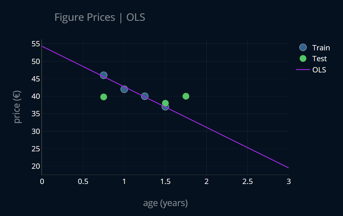
We then split our dataset into a train set and a test set, and trained our linear regression (OLS regression) model on the training data. Here’s how that looked like:

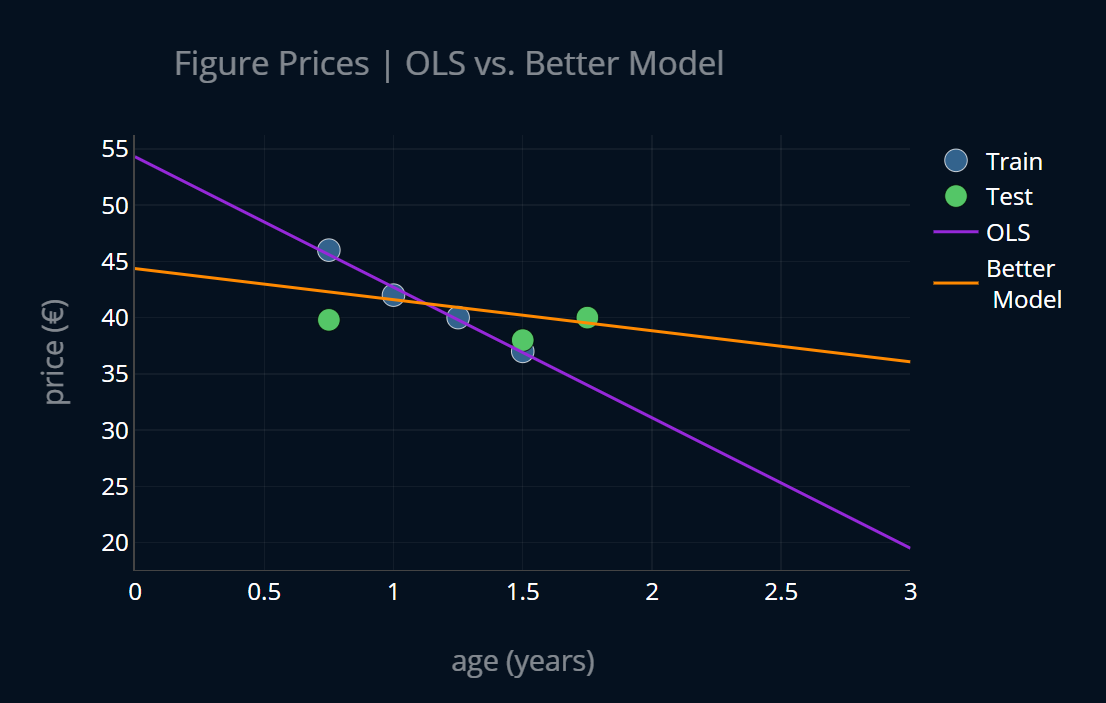
We then noticed that this model had a very low training error but a rather high testing error and thus we concluded that our linear regression model is overfit. We then tried to come up with an imaginary, better model that was less overfit and looked more like this:

This imaginary model turned out to be ridge regression. We analyzed what exactly lead to our linear regression model overfitting and we noticed that the main cause of overfitting were large model parameters. After discovering this insight, we developed a new loss function that penalizes large model parameters by adding a penalty term to our mean squared error. It looked like this (where is the number of model parameters):
There’s just one problem with this loss function. Since our model parameters can be negative, adding them might decrease our loss instead of increasing it. In order to circumvent this, we can either square our model parameters or take their absolute values:
The first function is the loss function of ridge regression, while the second one is the loss function of lasso regression.
Elastic Net
What we can do now is combine the two penalties, and we get the loss function of elastic net:
And that’s pretty much it! Instead of one regularization parameter we now use two parameters, one for each penalty. controls the L1 penalty and controls the L2 penalty. We can now use elastic net in the same way that we can use ridge or lasso. If , then we have ridge regression. If , we have lasso. Alternatively, instead of using two -parameters, we can also use just one and one L1-ratio-parameter, which determines the percentage of our L1 penalty with regard to . So if and L1-ratio = 0.4, our L1 penalty will be multiplied with 0.4 and our L2 penalty will be multiplied with . Here’s the equation:
Ok, looks good! In this case we have ridge regression if L1-ratio = 0 and lasso regression if L1-ratio = 1. In most cases, unless you already have some information about the importance of your features, you should use elastic net instead of lasso or ridge. You can then use cross-validation to determine the best ratio between L1 and L2 penalty strength. Now let’s look at how we determine the optimal model parameters for our elastic net model.
Solving Elastic Net
If L1-ratio = 0, we have ridge regression. This means that we can treat our model as a ridge regression model, and solve it in the same ways we would solve ridge regression. Namely, we can use the normal equation for ridge regression to solve our model directly, or we can use gradient descent to solve it iteratively.
If L1-ratio = 1, we have lasso regression. Then we can solve it with the same ways we would use to solve lasso regression. Since our model contains absolute values, we can’t construct a normal equation, and neither can we use (regular) gradient descent. Instead, we can use an adaptation of gradient descent like subgradient descent or coordinate descent.
If we are using both the L1 and the L2-penalty, then we also have absolute values, so we can use the same techniques as the ones we would use for lasso regression, like subgradient descent or coordinate descent.
Implementing Elastic Net Regression
If you’re interested in implementing elastic net from scratch,
then I recommend that you take a look at the articles about subgradient descent or coordinate descent,
where we do exactly that! In this article, we will use scikit-learn to help us out.
Scikit-learn provides a ElasticNet-class, which implements coordinate descent under the hood.
We can use it like this:
elastic_pipeline = make_pipeline(StandardScaler(),ElasticNet(alpha=1, l1_ratio=0.1))elastic_pipeline.fit(X_train, y_train)print(elastic_pipeline[1].intercept_, elastic_pipeline[1].coef_)# output: 41.0 [-1.2127174]
Just like with lasso,
we can also use scikit-learn’s SGDRegressor-class, which uses truncated gradients instead of regular ones.
Here’s the code:
elastic_sgd_pipeline = make_pipeline(StandardScaler(), SGDRegressor(alpha=1, l1_ratio=0.1, penalty = "elasticnet"))elastic_sgd_pipeline.fit(X_train, y_train)print(elastic_sgd_pipeline[1].intercept_, elastic_sgd_pipeline[1].coef_)# output: [40.69570804] [-1.21309447]
Cool! In practice, you should probably stick to ElasticNet instead of SGDRegressor since
coordinate descent converges more quickly than the truncated SGD in this scenario.
Since we’re using regularized models like lasso or elastic net it is important to first standardize our data before feeding it into our regularized model! If you’re interested in what happens when we don’t standardize our data, check out When You Should Standardize Your Data. There you will learn all about standardization as well as pipelines in scikit-learn, which is what we’ve used in the above code to make our lives a bit easier.
Parameter Sparsity Testing for Elastic Net
The most important property of lasso is that lasso produces sparse model weights, meaning weights can be set all the way to 0. Whenever you are presented with an implementation of lasso (or any model that incorporates an L1-penalty, like elastic net), you should verify that this property actually holds. The easiest way to do so is to generate a randomized dataset, fit the model on it, and see whether or not all of the parameters are zeroed-out. Here it goes:
elastic_rand_pipeline = make_pipeline(StandardScaler(),ElasticNet(alpha=1, l1_ratio=0.1))elastic_rand_pipeline.fit(X_rand, y_rand)print(elastic_rand_pipeline[1].intercept_, elastic_rand_pipeline[1].coef_)# output:# 0.4881255425051216 [-0. 0. -0. -0. -0. -0. -0. -0. -0. 0. -0. 0. -0. -0. 0. 0. -0. -0.# -0. 0. -0. 0. -0. -0. 0. -0. 0. 0. 0. -0. -0. 0. -0. -0. 0. 0.# -0. 0. -0. -0. 0. 0. 0. 0. -0. 0. 0. 0. -0. -0.]
Nice, the weights are all zeroed out!
We can perform the same test for SGDRegressor:
elastic_sgd_rand_pipeline = make_pipeline(StandardScaler(), SGDRegressor(alpha=1, l1_ratio=0.1, penalty = "elasticnet"))elastic_sgd_rand_pipeline.fit(X_rand, y_rand)print(elastic_sgd_rand_pipeline[1].intercept_, elastic_sgd_rand_pipeline[1].coef_)# output:# [0.46150165] [0. 0. 0. 0. 0. 0. 0. 0. 0. 0. 0. 0. 0. 0. 0. 0. 0. 0. 0. 0. 0. 0. 0. 0.# 0. 0. 0. 0. 0. 0. 0. 0. 0. 0. 0. 0. 0. 0. 0. 0. 0. 0. 0. 0. 0. 0. 0. 0.# 0. 0.]
Nice!
Finding the optimal value for and the L1-ratio
Here, we can use the power of cross-validation to compute the most optimal
parameters for our model. Scikit-learn even provides a special class for this
called ElasticNetCV. It takes in an array of -values to compare and select
the best of. If no array of -values is provided, scikit-learn will automatically
determine the optimal value of . We can use it like so:
elastic_cv_pipeline = make_pipeline(StandardScaler(),ElasticNetCV(l1_ratio=0.1))elastic_cv_pipeline.fit(X_train, y_train)print(elastic_cv_pipeline[1].alpha_)# output: 0.6385668121344372
Ok that’s nice, but how can you find an optimal value for the L1-ratio?
ElasticNetCV only determines the optimal value for , so if we want to
determine the optimal value for the L1-ratio as well, we’ll have to do an additional round
of cross-validation. For this, we can use techniques such as grid or random search,
which you can learn more about by reading the article Grid and Random Search Explained, Step by Step.
A Summary of Scikit-Learn-Classes
We’ve looked at quite a few models so far. To make it easier to remember when you should use which scikit-learn-class, I’ve created this little table. Here you can find the corresponding scikit-learn class for every model and every solver. This should make it a bit more organized.
| Model / Solver | Normal Equation | Gradient Descent variant |
|---|---|---|
| OLS Regression | LinearRegression | SGDRegressor [SGD] |
| Ridge | Ridge | SGDRegressor with penalty=“l2” [SGD] |
| Lasso | / | Lasso [Coordinate Descent] or SGDRegressor with penalty=“l1” [Truncated SGD] |
| Elastic Net | / | ElasticNet [Coordinate Descent] or SGDRegressor with penalty=“elasticnet” [Truncated SGD] |
Further Reading
We’ve looked at ridge, lasso, and elastic net in the context of regression, but we can also take the corresponding penalties and apply them to other models, like logistic regression or polynomial regression, as well. If you’re interested in these regularized models, I recommend you take a look at the articles Logistic Regression Explained, Step by Step and Polynomial Regression Explained, Step by Step respectively. In those articles you will learn everything about the named models as well as their regularized variants!
Classes like RidgeCV, LassoCV or ElasticNetCV are handy,
but not every model has a CV-variant. But if you know how cross-validation works,
you can make these models yourself! Cross-validation is an extremely important method
to train machine learning models effectively and to optimize hyperparameters.
You can read more about this technique in the article Cross-Validation Explained, Step by Step,
where you will learn everything you need to know to start using cross-validation in your own projects!
Share on:
