Bias, Variance, and Overfitting Explained, Step by Step
You have likely heard about bias and variance before. They are two fundamental terms in machine learning and often used to explain overfitting and underfitting. If you're working with machine learning methods, it's crucial to understand these concepts well so that you can make optimal decisions in your own projects. In this article, you'll learn everything you need to know about bias, variance, overfitting, and the bias-variance tradeoff.
Share on:
Background image by Sora Shimazaki (link)
Outline
Bias and variance are very fundamental, and also very important concepts. Understanding bias and variance well will help you make more effective and more well-reasoned decisions in your own machine learning projects, whether you’re working on your personal portfolio or at a large organization. In this article, you will learn what bias and variance are, what the so-called bias-variance tradeoff is, and how you can make the best decisions in your own machine learning projects, to create the best-performing machine learning models.
The Problem
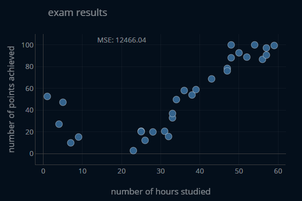
Let’s start by looking at a particular scenario. Imagine you are teaching your friend the basics of machine learning. You give them a small dataset of exam results. Each entry in the dataset contains the number of hours a student has spent studying for the exam as well as the number of points (between 0 and 100) the student has achieved in said exam. You then tell your friend to try and predict the number of points achieved based on the number of hours studied. The dataset looks like this:
Your friend is just getting started with machine learning and recently read an article about linear regression. Now they want to try out linear regression themselves! After some time, they come back to you and say that they have had difficulty creating a model that achieves a low error. You take their model and make a series of predictions. Then, you plot those predicted values alongside the actual exam scores for every number of hours studied in the dataset. To make the visuals easier to digest, the predictions are displayed as a continuous function. The resulting plot looks like this:
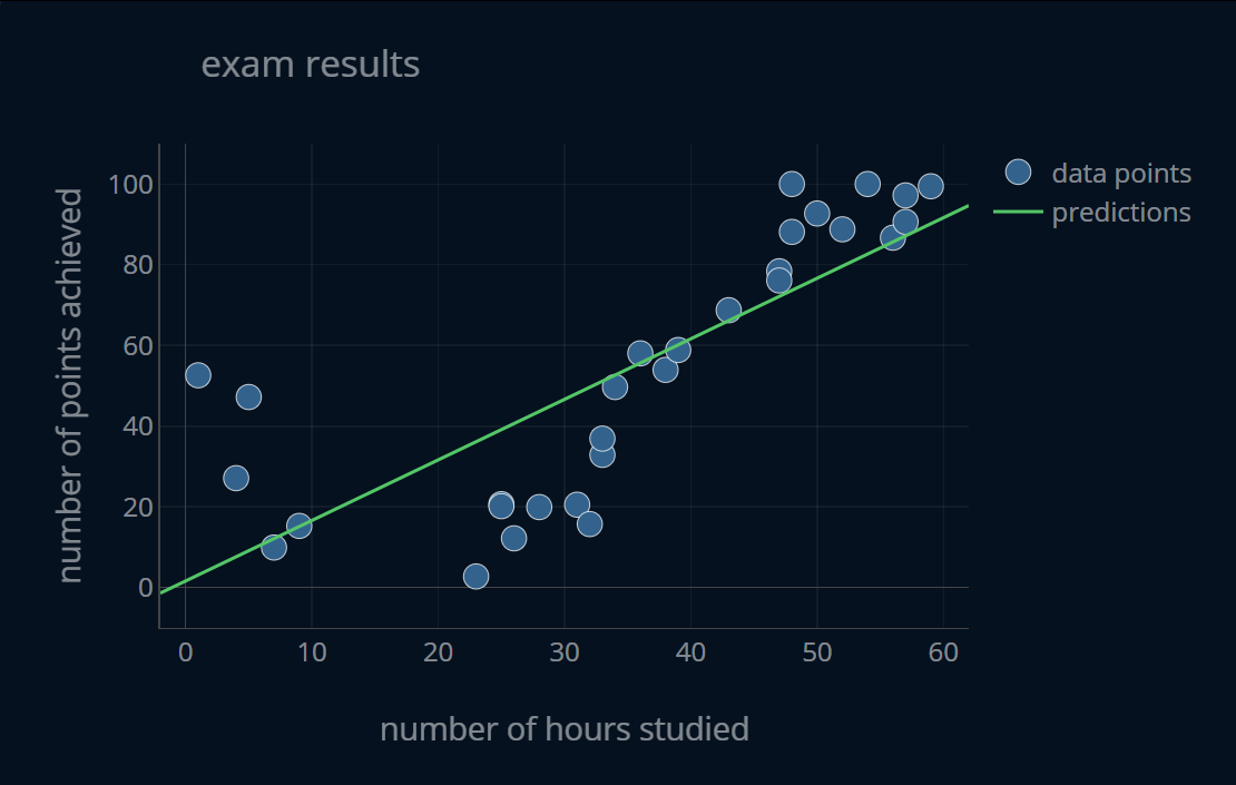
You look at the plot and notice a couple of things.
There definitely seems to be a relationship between the number of hours studied and the number of points achieved.
This relationship does seem somewhat linear, especially when considering the segment between 40 and 60 hours studied.
However, the linear relationship is not that apparent throughout the entire graph. When you take a look at the interval between 0 and 30 hours studied, it does seem to have more of a downward trend, in contrast to the interval between 40 and 60 hours studied.
With linear regression, we can only draw a straight line (a linear function) to model the relationship between the two features (number of hours studied) and the target (number of points achieved). But the data does not seem to follow the same trend throughout the entire dataset. We can’t just cut off one half of the dataset, so what can we do instead? In this case, we need to use a different model. No plain linear regression model can capture this relationship well. However, we can perform a small adjustment and use polynomial regression instead. With this, we can capture nonlinear relationships in our data using polynomial functions, instead of just linear ones. You explain this idea to your friend and they go ahead and try out polynomial regression.
Imagine you are in the shoes of your friend right now. You have to find out the degree of your polynomial regression model, meaning the maximum power which you will apply to your features. Is a degree of 2 or 3 already enough? Do you need a degree of 10 or higher? Pause for a second and think about this question. Below you can find an interactive visualization where you can take a look at all the possible polynomial regression plots for the degrees 1-20. After you’ve come up with a number in your head, take a look at the visualization and see if your intuition was right.
If you estimated the optimal degree to be between 3 and 5, congratulations! You’ve hit the gold spot. We, with our human eyes, can tell that the model with a degree between 3 and 5 best fits the data. But what’s interesting is that by increasing the degree of our polynomial regression model, our function always gets closer and closer to our data points. F.e. the model with degree 20 is touching a lot more points directly in the middle than the function with degree 3. The higher our degree is, the “wigglier” our function can get. Because a model with a higher degree has more degrees of freedom, it can take on more complicated function shapes. So maybe the model with degree=20 is truly the best one? Ok, let’s take a step back.
We have all of these different functions and some can capture the relationship between our features and our target better than others. If we were to compare the models with degree=1 and degree=20 respectively, we would say that the one with degree=20 “captures the relationship better”. But in a practical scenario, there has to be a better way of expressing this without having to say “captures this relationship better” every time. Wouldn’t it be more satisfying if we could somehow say that the model with degree=20 has a higher/lower something than the model with degree=1? We can do exactly that by introducing the notion of bias.
The Bias
We want the bias to express how well a certain machine learning model fits a particular dataset. So let’s try and come up with a formal definition of bias ourselves and look at some examples. Then, we will take a look at how the bias is defined in statistics and whether our own definition matches the one from statistics. Our definition might look similar to this:
The bias of a specific machine learning model trained on a specific dataset describes how well this machine learning model can capture the relationship between the features and the targets. So for our example, the bias of any one model would tell us how well this particular model can predict the exam points received for any number of hours studied in our specific dataset.
That seems like a reasonable definition.
Practical Examples (Bias)
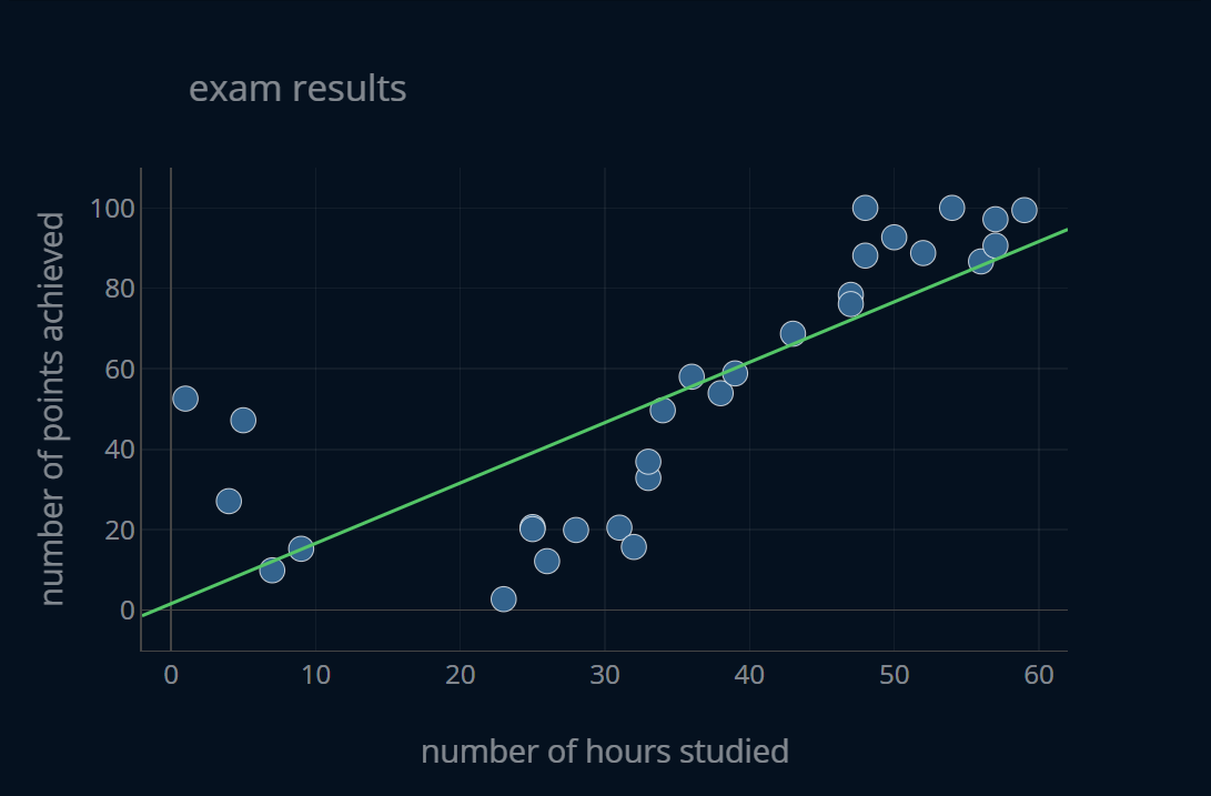
Let’s take a look at three of the above models and compare them using our new definition of bias. We’ll take a look at the polynomial regression models with degrees 1,4, and 15 respectively. Below is the graph showing our dataset and the predictions of the model with a degree of 1.
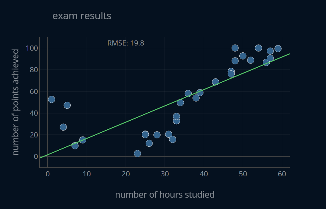
As you see, this model predicts our targets very poorly. The predicted values are not that close to the data points and therefor we can say that this model has a very high bias because it does not perform its task well, which is to predict the number of points achieved based on the number of hours studied.
In practice, we probably don’t want to generate a fancy graph displaying our predictions and then estimate how high our bias is based on how “good” the generated graph is. If we want to compare two models, then there has to be a more concrete way of measuring the bias. This is why in practice, we often use the (training) error
If we compute the root mean squared error (RMSE) for the predictions of this model, we get a value of 19.8. This means that one single point can be off by up to ~19.8, i.e. if a student in truth achieved 80 points, our model might only give them 60, which would probably not make the student very happy. With this we can capture the following behavior:
- large training error -> large bias
Let’s now look at the model with degree 4:
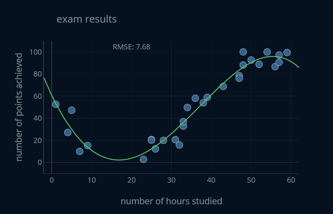
This model predicts our y a lot better than the first one. It still makes some errors, but it does its job a lot better than the first model. If we compute the RMSE for the predictions of this model, we get 7.68. It’s about 2.5 times better than the previous model! If a student in truth achieved 80 points, our model might only give them 72 (or up to 88), which still is not ideal, but it’s considerably better than the previous model. We achieved this decrease in error by just moderately increasing our degree. We’ve only increased the degree from 1 to 4, but managed to reduce our error by a factor of around 2.5! So this increase in complexity was certainly worth it. Because our model has a rather small error, we can say that it has a small bias since it does its task relatively well. With this we can capture the following behavior:
- small training error -> small bias
Let’s now take a closer look at the model with degree 15:
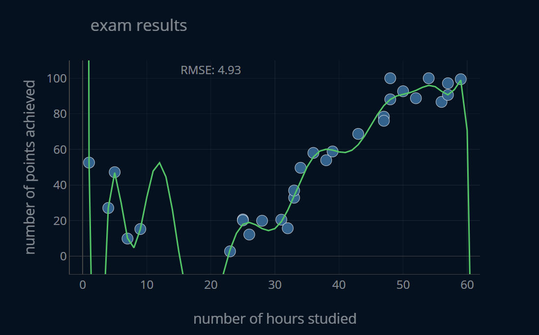
This model does look a bit weirder than the previous two, but it does in fact predict our data even better than the second one. If we compute the RMSE for the predictions of this model, we get 4.93. It’s about 1.5 times lower than the previous error. However, we did increase our degree from 4 to 15, which is quite a lot. So this increase in complexity certainly is not as good of a deal as the previous one. But a lower is a lower error, right? So technically, this model is the best of the bunch.
Because our model has a very low error, we can say that it has a very low bias since it does its task very well. With this we can capture the following behavior:
- very small training error -> very small bias
Revisiting the Definition of Bias
Ok, so we have defined the bias in our own words, we’ve looked at a couple of examples and we know that the training error is correlated with the bias. The lower the training error, the lower the bias. The higher the training error, the higher the bias.
When talking about the bias of a particular model, we always talk about one model and one dataset. In our case, we’ve always talked about one particular polynomial regression model and one particular dataset of exam results.
Let’s now look at the definition used in statistics and then try to see if our previous definition still holds. In the words of Wikipedia:
Statistical bias is a feature of a statistical technique or of its results whereby the expected value of the results differs from the true underlying quantitative parameter being estimated.
If we look back on how we introduced the bias, this makes sense. We compared the predictions of our model with the actual values present in our dataset. But the real definition is worded just a tiny bit differently, and contains two very important words:
Statistical bias is a feature of a statistical technique or of its results whereby the expected value of the results differs from the true underlying quantitative parameter being estimated.
This means that the bias is a way of describing the difference between the actual, true relationship in our data, and the one our model learned. In our examples, we’ve looked at the error between our predictions and the data points. Sure, that is a very sensible way to measure the bias of our machine learning models. But what guarantees that our dataset accurately represents the true relationship between our features and the target? Well, nothing. Our dataset can contain noise, meaning that, even if we could compute the true relationship of our data, the points would not lie directly on it. Since I’ve created this dataset myself using a specific function
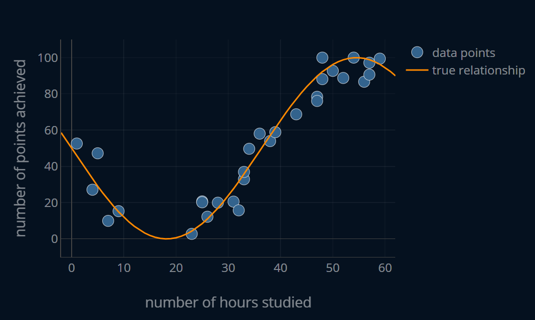
If the dataset contains no noise at all, it means that the dataset represents the exact underlying relationship. But almost every dataset out there will have some noise in it. This might be because the dataset was not properly cleaned, or maybe because there is some intrinsic noise to the underlying problem itself. Often times it is simply not possible to get perfect, noiseless data. For this reason, there might be an irreducible error, an error, that no machine learning model (or even human) can undergo. So if the definition of bias from statistics compares the predicted relationship with the true, underlying relationship, why don’t we do the same as well? Because oftentimes, we simply can’t.
I can show you how this exemplary dataset looks like without the noise because I generated the dataset using a mathematical function. However, real datasets are often sampled from actual events, which may or may not follow the shape of some mathematical function. So most of the time, it’s exactly the opposite of the scenario presented here. We usually have a seemingly random dataset and we want to create a mathematical function that models a certain relationship in that dataset. Here, I’ve done the opposite. I’ve created a function and then generated a random dataset using that function. If this dataset was truly random, we would have no way of knowing how much noise it contains or what part of the dataset really is noise.
This is the reason why we compare our dataset to our predictions. Ideally, we want our function to learn this true, underlying relationship, by only looking at the noisy dataset. Almost always we won’t be able to create a model that perfectly matches this relationship (and we also don’t have a way of checking if it did), but oftentimes we can generate a function that is good enough, assuming the dataset itself is good enough. So what does this mean? If our model creates a relationship that we think is not as sensible, 4/5 times it will be the dataset that is to blame, and not the model.
But how do we tell if our model is good?
Naturally, we are interested in keeping the bias as low as possible, because we want our model to make the best predictions possible. But if you take a look at the second and third model, would you really choose the third model over the second one? It does have a lower bias, so this is certainly an argument. But there is just something off about the third model. Maybe it’s the fact that it looks a lot less “stable” than the second one. Maybe it’s the fact that it just seems a little too good at its task. But let’s not get ahead of ourselves. There has to be a way to tell whether the third model really is not so great, or whether it’s truly the best of the bunch. And to do this, we are now going to take a look at the notion of variance.
The Variance
With the bias, we now have a way of expressing how well a machine learning model can represent the relationship between feature and target values. Now, with the bias, we always only consider one dataset, but what would happen if we bring in values our model has not seen before? What happens when we bring in another dataset? Obviously, we won’t consider a dataset of apples and oranges if our model was trained to predict exam scores, but what if we bring in a dataset that is very similar
We want the variance to express how consistent a certain machine learning model is in its predictions when compared across similar datasets. So let’s apply the same approach that we used for the bias and try to first come up with a formal definition of variance ourselves. It might look like the definition below.
The variance of a specific machine learning model trained on a specific dataset describes how much the performance of the machine learning model differs when evaluated on different datasets of the same origin. So for our example, the variance of any one model would tell us how robust the performance of this particular model is, meaning if we were to slightly change the values of our data points, how much would our performance fluctuate?
Ok, now let’s take a look at the same three polynomial regression models that we analyzed previously.
Practical Examples (Variance)
This time, I’ll add a function to each plot that slightly alters the dataset when clicked. Let’s also display some additional information. First, we will display the RMSE for that particular model and the (potentially altered) dataset. Second, we will also track the relative difference (R.DIFF) between the current MSE and the initial MSE.
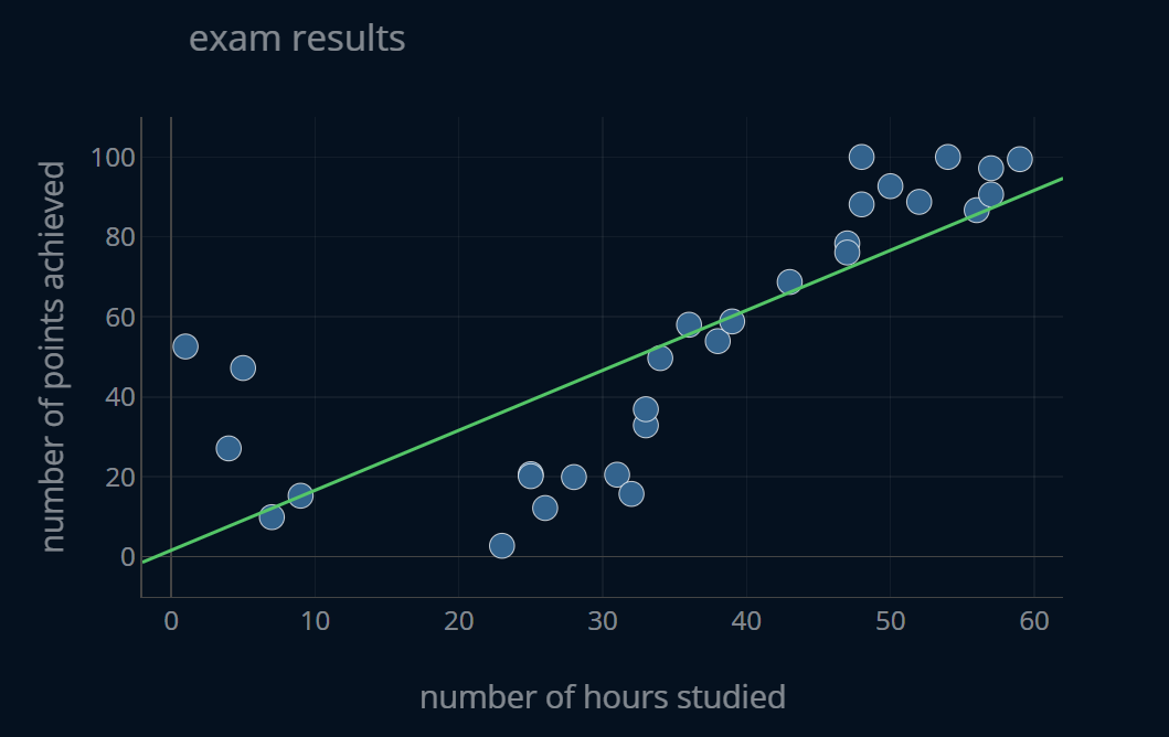
This model predicts our y very poorly. This poor performance is also maintained if we slightly alter the dataset. If you press the button a couple of times and keep an eye on the RMSE and the R.DIFF, you’ll notice that the values don’t change that much. To be more exact, if you compute the average relative difference of 1000 RMSE values for slightly altered datasets, you will receive a value of ~1.7. This means that, if we slightly change our dataset, our MSE will fluctuate by around 1.7%, which makes the model very consistent. In other terms, our model performs poorly, and does so consistently. It always makes bad predictions for a dataset of this origin. Because the performance of this model is very consistent across multiple similar datasets, we can say that it has a very low variance.
With this we can capture the following behavior:
- small fluctuation of the error -> small variance
In practice, we usually don’t want to randomly alter our dataset and keep track of the relative difference to find out whether our variance is low or high. So how can we estimate the variance of a machine learning model? We look at the difference in performance between the training-set and the testing-set (or for that matter, the training set and any other dataset of similar origin). If this difference is high, so is the variance. If it is low, so is the variance.
Because the model with degree=1 has a high bias but a low variance, we say that it is underfitting, meaning it is not “fit enough” to accurately model the relationship between features and targets.
Let’s now look at the model with degree 4:
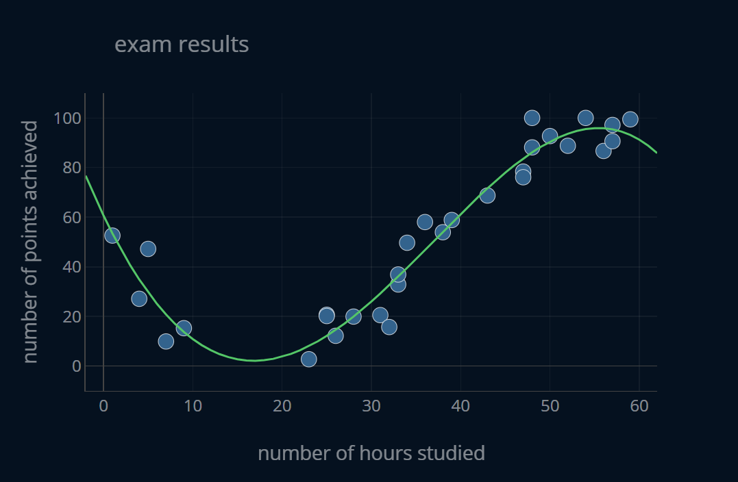
This model predicts our y a lot better than the first one. This good performance is also somewhat stable if we alter the dataset. If you again press the button a couple of times and keep an eye on the RMSE and the R.DIFF, you’ll notice that the values change a little bit, but not a lot. To be more exact, if you compute the average relative difference of 1000 RMSE values for slightly altered datasets, you will receive a value of ~13.6. This means that if we slightly change our dataset, our MSE will fluctuate by around 13.6%, which makes the model somewhat consistent. It’s certainly not as consistent as the first model, but it’s not terrible as well. In other terms, our model performs well, and does so pretty consistently. It always makes at least decent predictions for a dataset of this origin. Because the performance of this model is somewhat consistent across multiple similar datasets, we can say that it has a somewhat low variance.
With this we can capture the following behavior:
- medium fluctuation of the error -> medium variance
Because the model with degree=4 has a low bias and a low variance, we say that it is well fit, meaning it has just the right balance between bias and variance.
Let’s now look at the model with degree 15:
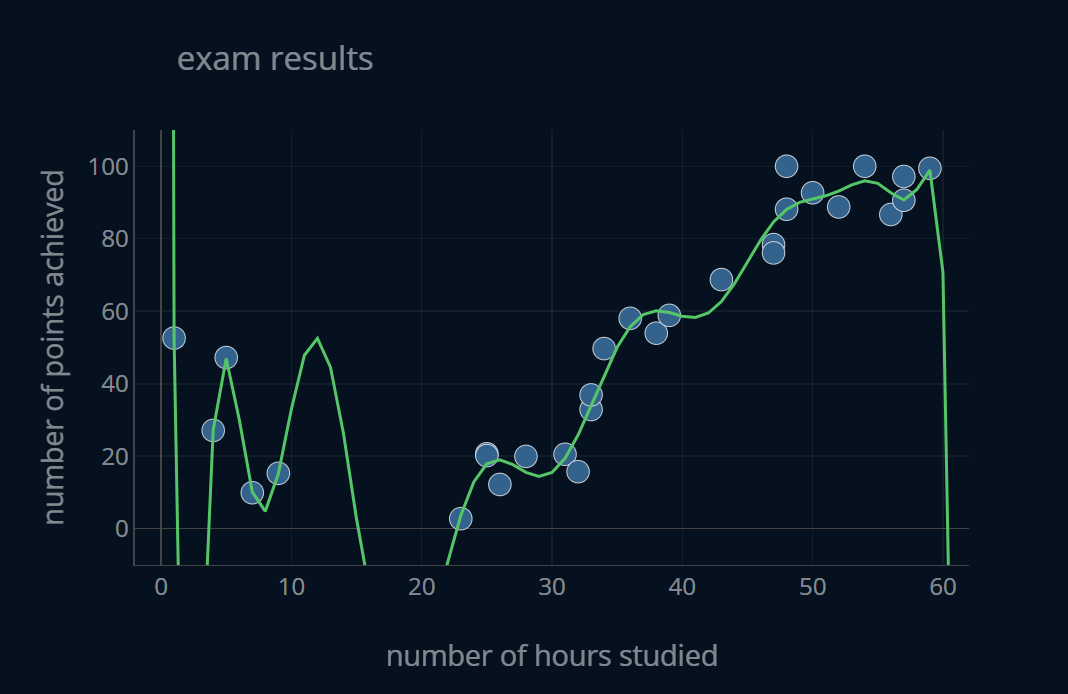
This model predicts our data very well. However, this outstanding performance is not at all maintained when we change up our dataset a bit. If you press the button just a few times and look at the RMSE and R.DIFF, chances are you’ll see some larger numbers than before. These numbers also change quite a lot between clicks. To be more exact, if you compute the average relative difference of 1000 RMSE values for slightly altered datasets, you will receive a value of ~169.5. 169.5! This means that if we slightly change our dataset, our RMSE will fluctuate by around 169.5%, which makes the predictions of this model as reliable as your office or home printer in the moment you need it most. This means that our model performs well sometimes, and catastrophically other times. Because the performance of this model is very inconsistent across multiple datasets, we can say that it has a high variance.
With this we can capture the following behavior:
- high fluctuation of the error -> high variance
Because this model has a low bias but a high variance, we say that it is overfitting, meaning it is “too fit” at predicting this very exact dataset, so much so that it fails to model a relationship that is transferable to a similar dataset.
Revisiting the Definition of Variance
Ok, so we have defined the variance, looked at examples, and we know that the error fluctuation is correlated with the variance. The lower the error fluctuation, the lower the variance. The higher the error fluctuation, the higher the variance.
When talking about the variance of a particular model, we always talk about one model, but multiple datasets. In practice, you would compare the model error on the training dataset and the error on the testing (or validation) dataset.
Let’s now also look at the definition used in statistics. In the words of Wikipedia:
In probability theory and statistics, variance is the expectation of the squared deviation of a random variable from its mean. In other words, it measures how far a set of numbers is spread out from their average value.
The important part is ”spread out from their average value”. This means that the variance is a way of describing the difference between the expected (or average) value and the predicted value of our model. This definition is similar to the one we described earlier.
Naturally, we are interested in keeping the variance as low as possible, because we want our model to make consistent predictions across all datasets. If we again take a look at the second (degree=4) and third (degree=15) model, we can see that the third model may have a lower bias than the second one, but it also has a lot higher variance when compared to the second model. Therefor, the second model is the overall best model out of the three, because it succeeds in minimizing both bias and variance at the same time, while the first model (degree=1) minimizes just the variance, and the third model minimizes just the bias.
The Tradeoff
Let’s think about how we might decrease bias. The easiest way to achieve a lower bias would be to pick a more complex model or to train our existing model for longer. In other words, we want to extract more insights from our dataset, we want our model to learn more from our data. The more our model learns from our data, the better it will be at solving its task.
And how might we decrease variance? The easiest way to decrease variance would be to pick a more simple model or to train our existing model for a shorter amount of time. In other words, we want to extract fewer insights from our dataset, we want our model to learn less from our data. The less our model learns from our data, the more general it will be, because it has only learned so much to base its predictions on.
A good analogy would be to think of a student preparing for their mathematics and physics exams. If the student does not prepare at all, they will do poorly in both exams (high bias). If they put a lot of time into their preparation, they will probably do pretty well in both exams (low bias, low variance). However, if the student puts a lot of time into their preparation, and does the same exercises over and over and over again (prolonged training on the same dataset), they will train themselves not to be good at solving math and physics exams, but to be good at solving those particular exercises they have solved over and over again. If they see a question on the exam that they have practiced, they will solve it without any error. However, if they see a question that they have not practiced, they will have a more difficult time answering it (low bias, high variance).
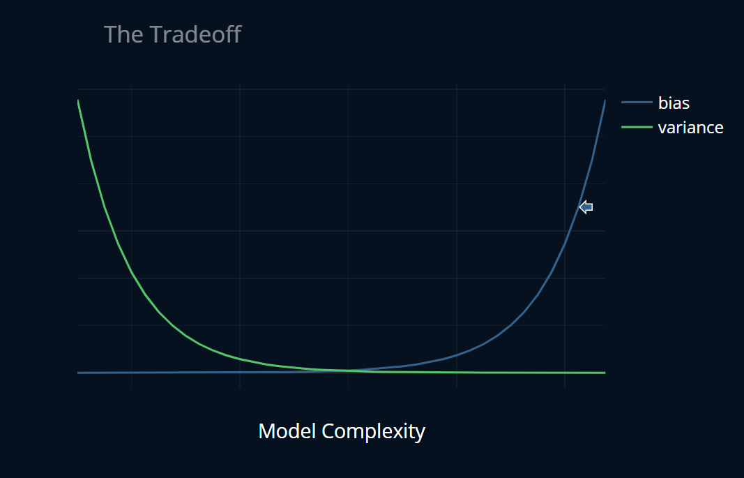
So there seems to be a sort of “tradeoff” between bias and variance. You can only decrease your bias so much until your variance starts to increase. At this point, you might think of a graph like this one:
The Tradeoff?
If you have a rather simple model like polynomial regression, there certainly is a tradeoff between bias and variance. As you saw, increasing the degree up to a specific point decreased bias considerably, while only slightly affecting variance. After that specific point, the variance just started to increase dramatically, rendering the further decrease in bias meaningless.
However, if you have a rather complicated model such as a deep neural network, things get a little bit more complicated. Oftentimes it seems as if the bias-variance tradeoff is not really such “tradeoff” in these cases anymore. I don’t want to get into too much detail here because this topic is extensive enough to fill a separate article. However, I do want to point you to some external resources if you are interested in reading more about this. There is this blog article by Brady Neal which explains the topic in an easy-to-follow fashion. If you are looking for a more rigorous source, consider reading the paper A Modern Take on the Bias-Variance Tradeoff in Neural Networks, whose first author is the same person who wrote the aforementioned blog post. The paper covers the topic a bit more in-depth.
An All-Purpose Remedy?
No matter what machine learning model you are training and which problem you are trying to solve, there is one thing you can do that will almost always result in a better, more stable machine learning model. What is it? Simply said, “getting more (and better) data”. There have been numerous papers written and studies performed
So what does this mean for you? If you are unsatisfied with the performance of your machine learning model, and you have already tried out a variety of parameter configurations and alternative models, then your 1# chance to increase model performance is to get more and better data. When your machine learning model is underperforming, the underlying issue is frequently present in the dataset itself, and not in the model.
Diving Deeper
In this article, I briefly talked about the concept of an irreducible error, an error, that is present in the problem/data itself, and that no machine learning model (or even human) can undergo. This is the reason why a training error of 0.15 might be amazing in one application, and horrible in another. Therefor it makes sense to remember this concept when you are analyzing the bias of a machine learning model. If your models have been stuck at a certain bias and don’t improve any further no matter what you do, it may just be the case that you’ve reached the ideal bias for this particular problem and that it is simply not possible to improve any further with this particular dataset that you have.
Oftentimes you won’t know the irreducible error for a problem. It is pretty difficult to compute and it’s even more difficult to prove that it really is irreducible. In practice, you can’t compute the irreducible error for every problem you try to solve with machine learning. What you can do instead, is to train multiple different machine learning models
Further Reading
Bias and variance are two terms that are often used to describe overfitting and underfitting. In this post, we saw what exactly over-and underfitting is, but how can you actually prevent it in practice? If you want to know how you can stop overfitting (and underfitting), then I recommend you read the post How To Stop Overfitting and Underfitting, where you will learn a variety of techniques that can help you make your model more robust against both overfitting as well as underfitting.
You can only improve your machine learning models so much until it becomes very difficult to improve their performance any further. However, oftentimes you will get even better results when you optimize the dataset your machine learning models are trained on. There are lots of ways with which you can improve your data, and if you want to learn how exactly you can do so, you should take a look at the section Dataset Optimization, where you will find many articles that explain exactly how you can do so.
Share on:
